Class 1: Python Refresher, Data Structures, Numpy#
Goal of today’s class:
Make sure we’re all on the same page with Python
Review the basics, discuss
types, operations, data structures
Demonstrate best practices for writing functions, both in notebook environments and as scripts
Start discussing the basics of data summarization + communication (
matplotlib)
Acknowledgement: Much of the material in this lesson is based on a previous course offered by Matteo Chinazzi and Qian Zhang.
Come in. Sit down. Open Teams.
Make sure your notebook from last class is saved.
Run
python3 git_fixer2.pyGithub:
git add … (add the file that you changed, aka the
_MODIFIEDone)git commit -m “your changes”
git push origin main
Python#
In this class, we’ll be coding in Python. There are several reasons for this, but probably most importantly it’s the one we know best (and the most commonly-used language in Network Science!). Python is a high-level general-purpose language that is object-oriented, has dynamic/strong typing, interpreted, and interactive. It’s also quite easy to learn and has the potential to create legible and ultimately reproducible code.
Object-oriented: object-oriented programming (OOP) is a type of software design where the coder defines the type of a data structure and types of operations (functions) that can be applied to the data structure. Everything in Python is an object, and almost everything has “attributes” and “methods” — also, everything is an object in the sense that it can be assigned to a variable or passed as an argument to a function.
Dynamic typing means that runtime objects (values) have a type, as opposed to static typing where variables have a type.
Strong typing means that the type of a value doesn’t suddenly change. A string containing only digits doesn’t magically become a number, as may happen in other languages (e.g. Perl). Every change of type requires an explicit conversion.
Interpreted: you don’t need to compile your code, as is the case in other languages.
Interactive: you can write and execute parts of your program while the program itself is already running.
Main Features#
(source: https://www.python.org/)
Uses an elegant syntax, making the programs you write easier to read.
Is an easy-to-use language that makes it simple to get your program working. This makes Python ideal for prototype development and other ad-hoc programming tasks, without compromising maintainability.
Comes with a large standard library that supports many common programming tasks such as connecting to web servers, searching text with regular expressions, reading and modifying files.
Python’s interactive mode makes it easy to test short snippets of code. There’s also a bundled development environment called IDLE.
Is easily extended by adding new modules implemented in a compiled language such as C or C++.
Can also be embedded into an application to provide a programmable interface.
Runs anywhere, including Mac OS X, Windows, Linux, and Unix.
Is free software in two senses. It doesn’t cost anything to download or use Python, or to include it in your application. Python can also be freely modified and re-distributed, because while the language is copyrighted it’s available under an open source license.
A variety of basic data types are available: numbers (floating point, complex, and unlimited-length long integers), strings (both ASCII and Unicode), lists, and dictionaries.
Python supports object-oriented programming with classes and multiple inheritance.
Code can be grouped into modules and packages.
The language supports raising and catching exceptions, resulting in cleaner error handling.
Data types are strongly and dynamically typed. Mixing incompatible types (e.g. attempting to add a string and a number) causes an exception to be raised, so errors are caught sooner.
Python contains advanced programming features such as generators and list comprehensions.
Python’s automatic memory management frees you from having to manually allocate and free memory in your code.
Additional Facts#
Python was conceived in the late 1980s, and its implementation was started in December 1989 by Guido van Rossum, the National Research Institute for Mathematics and Computer Science in the Netherlands (CWI) and had originally focused on users as physicists and engineers.
Python was designed from another existing language at the time, called ABC.
The name Python was taken by Guido van Rossum from british TV program Monty Python Flying Circus and there are many references to the show in language documentation.
The goals of the Python project were summarized by Tim Peters in a text called Zen of Python :
Fun…#
import this
The Zen of Python, by Tim Peters

Beautiful is better than ugly.
Explicit is better than implicit.
Simple is better than complex.
Complex is better than complicated.
Flat is better than nested.
Sparse is better than dense.
Readability counts.
Special cases aren't special enough to break the rules.
Although practicality beats purity.
Errors should never pass silently.
Unless explicitly silenced.
In the face of ambiguity, refuse the temptation to guess.
There should be one-- and preferably only one --obvious way to do it.
Although that way may not be obvious at first unless you're Dutch.
Now is better than never.
Although never is often better than *right* now.
If the implementation is hard to explain, it's a bad idea.
If the implementation is easy to explain, it may be a good idea.
Namespaces are one honking great idea -- let's do more of those!
# import antigravity
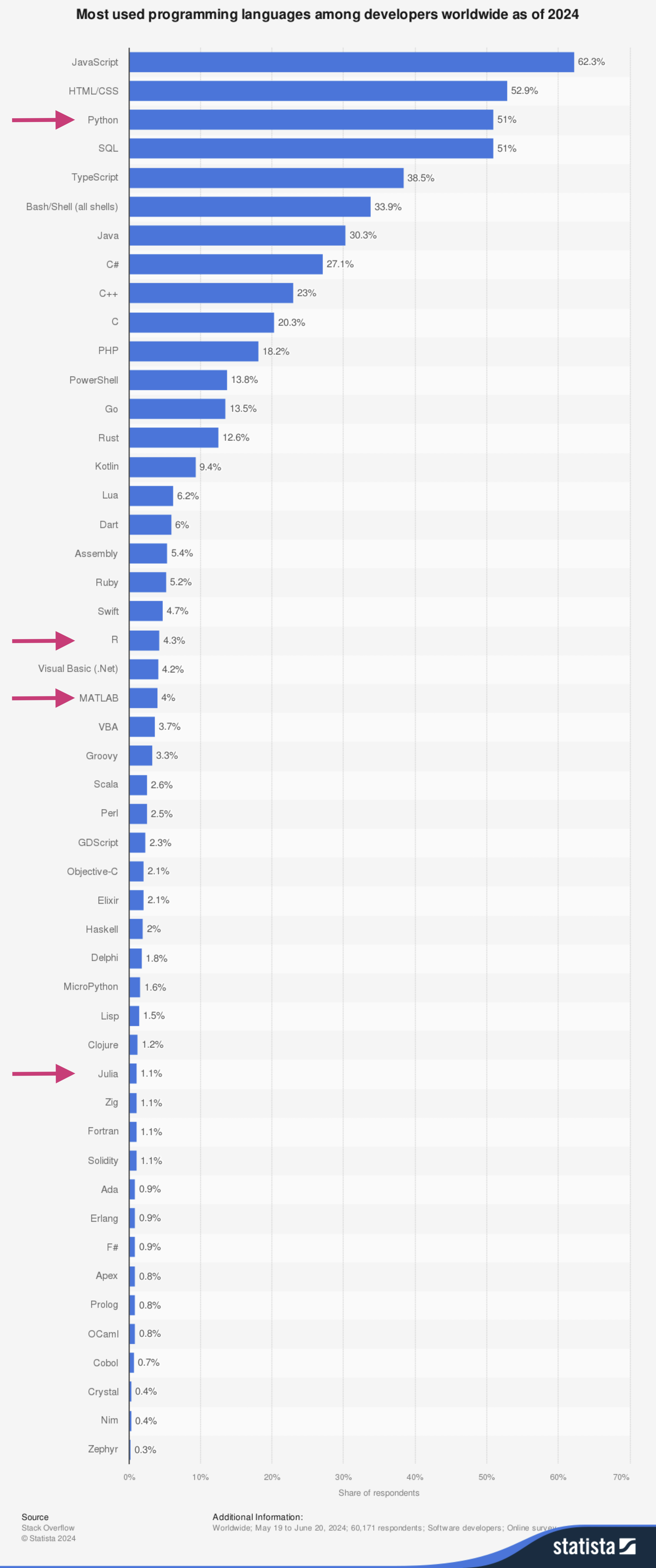
Python Today#
Source: https://www.statista.com/statistics/793628/worldwide-developer-survey-most-used-languages/
Additional Tools#
Jupyter Notebook (https://jupyter.org/) [already installed with Anaconda]
VS Code (https://code.visualstudio.com/) or any other text editor you might prefer such as Vim, Sublime, etc..
Commonly-used Software Libraries#
(most of them are already included in Anaconda)
numpy (https://numpy.org/)
scipy (https://www.scipy.org/)
matplotlib (https://matplotlib.org/)
seaborn (https://seaborn.pydata.org/)
pandas (https://pandas.pydata.org/)
beautifulsoup (https://www.crummy.com/software/BeautifulSoup/)
selenium (https://selenium-python.readthedocs.io/)
Additional Resources#
The Unix Shell (https://swcarpentry.github.io/shell-novice/)
Version Control with Git (https://swcarpentry.github.io/git-novice/)
Databases and SQL (https://swcarpentry.github.io/sql-novice-survey/)
A gallery of interesting Jupyter Notebooks (jupyter/jupyter)
‘Sup, world?#
Part 1: Very Basics#
print("Hello, World!")
Hello, World!
print("Hello", "World!")
Hello World!
range?
# print "hello, world!"
Part 2: Variables#
Variables in the Python interpreter are created by assignment.
Variable names must start with letter or underscore (
_) and be followed by letters, digits or underscores (_).Uppercase and lowercase letters are considered different (i.e., Python is case-sensitive).
a = 2
b = 4
x = "hello"
# Printing
print("a + b =",a + b)
print("a - b =",a - b)
print("a / b = %.2f"%(a/b))
print("a / b = {:f}".format(a/b))
print(f'a^b = {(a**b):d}')

print('\n')

print(x + x + x)
print(x * a)

print(x + x + str(a))
print(x + x + str(a**b))
a + b = 6
a - b = -2
a / b = 0.50
a / b = 0.500000
a^b = 16


hellohellohello
hellohello
hellohello2
hellohello16
whos
Variable   Type      Data/Info
------------------------------
a          int       2
b          int       4
this       module    <module 'this' from '/opt<...>/lib/python3.11/this.py'>
x          str       hello
del x
whos
Variable   Type      Data/Info
------------------------------
a          int       2
b          int       4
this       module    <module 'this' from '/opt<...>/lib/python3.11/this.py'>
print(type(a))
print(type(b))

b = a * 1.5
print(type(b))

x = "hello"
print(type(x))
<class 'int'>
<class 'int'>
<class 'float'>
<class 'str'>
Scope of Variables#
Not all variables are accessible from all parts of our program, and not all variables exist for the same amount of time. Where a variable is accessible and how long it exists depend on how it is defined. We call the part of a program where a variable is accessible its scope, and the duration for which the variable exists its lifetime.
A variable that is defined in the main body of a file is called a global variable. It will be visible throughout the file, and also inside any file that imports that file. Global variables can have unintended consequences because of their wide-ranging effects, which is why we should be careful about using them.
A variable that is defined inside a function is local to that function. It is accessible from the point at which it is defined until the end of the function, and exists for as long as the function is executing. The parameter names in the function definition behave like local variables, but they contain the values that we pass into the function when we call it. When we use the assignment operator (=) inside a function, its default behaviour is to create a new local variable, unless a variable with the same name is already defined in the local scope.
(source: https://python-textbok.readthedocs.io/en/1.0/Variables_and_Scope.html)
Part 3: Types in Python#
Text Type:
strNumeric Types:
int,float,complexSequence Types:
list,tuple,rangeMapping Type:
dictSet Types:
set,frozensetBoolean Type:
boolBinary Types:
bytes,bytearray,memoryviewNone Type:
NoneType
We’ll be working most with:
A) Booleans are either
TrueorFalse(case sensitive)B) Numbers can be integers (e.g
1or2), floats (1.1and1.2), fractions (1/2and2/3), or even complex numbers.C) Lists are ordered sequences of values, defined by its elements
[...].D) Strings are sequences of Unicode characters (e.g. an html document,
'eioajfwo', etc.).E) Tuples are ordered, immutable sequences of values (e.g.
(0,1)).F) Sets are unordered bags of values, defined using squiggly braces
{}.G) Dictionaries are unordered bags of key-value pairs (also defined with the squiggs, but requires
{key:value}).H) Bytes and byte arrays, e.g. a jpeg image file.
(A) Booleans#
Booleans are either true or false and in Python we can assign “boolean values” to variables using two constants: “True” and “False”.
True
True
False
False
True + True
2
True * 3
3
(B) Numbers#
# integers
print(1)

# floats
print(3.14)

# scientific notation
print(3.14e2)

# fractions
from fractions import Fraction
print(Fraction('1/2'))
print(Fraction('1/2') + 0.5)

print(Fraction('1/2') + Fraction('1/4'))
print(Fraction(1,2) + Fraction(1,4))


# complex numbers
c = 1 + 5j
type(c)

print(c.real)
print(c.imag)
print(c.conjugate())
1
3.14
314.0
1/2
1.0
3/4
3/4
1.0
5.0
(1-5j)
# cast from float to int
int(3.7)
3
# cast from int to float
float(3)
3.0
print(c)
(1+5j)
c.real?
Common Operations with Numbers:#
Sum (+)
Difference (-)
Multiplication (*)
Floating Point Division (/)
Integer Division (//): the result is truncated to the next lower integer, even when applied to real numbers, but in this case the result type is real too.
Module (%): returns the remainder of the division.
Power (
**): can be used to calculate the root, through fractional exponents (eg100 ** 0.5).Positive (+)
Negative (-)
Logical Operations:#
Less than (<)
Greater than (>)
Less than or equal to (<=)
Greater than or equal to (>=)
Equal to (==)
Not equal to (!=)
from IPython.display import display, Math

# sum
print("1 + 3 =",1+3)

# difference
display(Math(r'2-5 = {}'.format(2-5)))

# multiplication
print(5*4,'\n')

# floating point division
print(5/3)

# integer division
print(5//3,'\n')

# notice:
print(-5/3)
print(-5//3,'\n')

# modulo (returns the remainder of a division)
print(5%3,'\n')

# exponentiation
display(Math(r'2^4 = {}'.format(2**4)))
1 + 3 = 4
20

1.6666666666666667
1

-1.6666666666666667
-2

2
Numbers & Booleans#
Zero values evaluate to False and non-zero values evaluate to True.
x = 0
if x:
    print("do something")
(C) Lists#
Lists are collections of heterogeneous objects, which can be of any type, including other lists. They are mutable and can be changed at any time. Lists can be sliced in the same way that the strings, but as the lists are mutable, it is possible to make assignments to the list items.
my_list = ['item 1', 'item 2', [4,5], 5 ,6]
my_list
['item 1', 'item 2', [4, 5], 5, 6]
my_list = [0,1,2,3,4,5,6,7,8]

# indexing
print(my_list[0])

# slicing
print(my_list[:4])
print(my_list[4:])

print(my_list[1:])
print(my_list[:2])

print(my_list[::1])
print(my_list[::2])
print(my_list[::3])

print(my_list[1:7:2])

print(my_list[-1])
print(my_list[-2])

print(my_list[::-1])

## notice that the return value from slicing is a new list
0
[0, 1, 2, 3]
[4, 5, 6, 7, 8]
[1, 2, 3, 4, 5, 6, 7, 8]
[0, 1]
[0, 1, 2, 3, 4, 5, 6, 7, 8]
[0, 2, 4, 6, 8]
[0, 3, 6]
[1, 3, 5]
8
7
[8, 7, 6, 5, 4, 3, 2, 1, 0]
my_list = my_list + [10,11]
my_list
[0, 1, 2, 3, 4, 5, 6, 7, 8, 10, 11]
my_list.extend([12,13])
my_list
[0, 1, 2, 3, 4, 5, 6, 7, 8, 10, 11, 12, 13]
my_list.insert(7,'dog')
my_list
[0, 1, 2, 3, 4, 5, 6, 'dog', 7, 8, 10, 11, 12, 13]
# search for values in a list
'dog' in my_list
True
my_list.count('dog')
1
my_list.index('dog')
7
# remove items from a list

my_list.remove('dog')
my_list
[0, 1, 2, 3, 4, 5, 6, 7, 8, 10, 11, 12, 13]
my_list.pop()
13
my_list
[0, 1, 2, 3, 4, 5, 6, 7, 8, 10, 11, 12]
my_list.pop(-3)
10
my_list
[0, 1, 2, 3, 4, 5, 6, 7, 8, 11, 12]
# sum the elements of an iterable (e.g. a list)
print(sum(my_list))

# find the maximum value of the elements of an iterable (e.g. a list)
print(max(my_list))

# find the minimum value of the elements of an iterable (e.g. a list)
print(min(my_list))

# get the length of an object (e.g. a list)
print(len(my_list))
59
12
0
11
my_list = ['random item']*10
my_list
['random item',
 'random item',
 'random item',
 'random item',
 'random item',
 'random item',
 'random item',
 'random item',
 'random item',
 'random item']
len(my_list)
10
if my_list:
    print("do something")
do something
Lists and Booleans#
An empty list is False, any list with at least one item is true regardless of the actual value of the items.
(D) Strings#
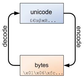
Strings are immutable: you can not add, remove, or change any character in a string. To perform these operations, Python needs to create a new string.
In Python 3, all strings are sequences of Unicode characters and can be encoded either as unicode objects or as bytes object.
Unicode is an international encoding standard for use with different languages and scripts, by which each letter, digit, or symbol is assigned a unique numeric value that applies across different platforms and programs.
j = '伯恩茅斯'
# length of a string
print("len(j) =",len(j))

print()
# access characters
for c in j:
    print(c)
len(j) = 4

伯
恩
茅
斯
j[2]
'茅'
x = j[2]
x
'茅'
j[2] = 'c'
---------------------------------------------------------------------------
TypeError                                 Traceback (most recent call last)
Cell In[44], line 1
----> 1 j[2] = 'c'

TypeError: 'str' object does not support item assignment
# formatting a string
s = '  heLlo, wOrld!  '

s.upper()
s.lower()
---------------------------------------------------------------------------
NameError                                 Traceback (most recent call last)
<ipython-input-45-32dd64412b48> in <module>
----> 1 s.lower()

NameError: name 's' is not defined
s.title()
Question: What does the following do?
# how to split a string
s.split()
s.split(',')
---------------------------------------------------------------------------
NameError                                 Traceback (most recent call last)
<ipython-input-46-2be51098b857> in <module>
----> 1 s.split(',')

NameError: name 's' is not defined
s.strip()
s.rstrip()
s.lstrip()
---------------------------------------------------------------------------
NameError                                 Traceback (most recent call last)
<ipython-input-47-e02c2e109a92> in <module>
----> 1 s.lstrip()

NameError: name 's' is not defined
String vs Bytes Objects#
ss = '伯恩茅斯'
ss
# encode a string
ss.encode()
---------------------------------------------------------------------------
NameError                                 Traceback (most recent call last)
<ipython-input-48-5ba7a394e7d4> in <module>
      1 # encode a string
----> 2 ss.encode()

NameError: name 'ss' is not defined
# encode + decode
ss.encode().decode()
# string lenght vs bytes length
print(len(ss.encode()))
print(len(ss))
UTF-8 encoding table and Unicode characters
https://www.utf8-chartable.de/
Note: Python 3 assumes that your source code (i.e., your .py file) is encoded in utf-8.
# from bytes to string
(b'\x7e').decode()
'~'
è = 10
e
---------------------------------------------------------------------------
NameError                                 Traceback (most recent call last)
<ipython-input-51-094e3afb2fe8> in <module>
----> 1 e

NameError: name 'e' is not defined
(E) Tuples#
Similar to lists, but immutable: its not possible to append, delete or make assignments to the items. Syntax:
my_tuple = (a, b, ..., z)
The parentheses are optional when defining a tuple.
Feature: a tuple with only one element is represented as:
t1 = (1,)
The tuple elements can be referenced the same way as the elements of a list:
first_element = tuple[0]
Lists can be converted into tuples:
my_tuple = tuple(my_list)
And tuples can be converted into lists:
my_list = list(my_tuple)
While tuple can contain mutable elements, these elements can not undergo assignment, as this would change the reference to the object.
Example (using the interactive mode):
>>> t = ([1, 2], 4)
>>> t[0].append(3)
>>> t
([1, 2, 3], 4)

>>> t[0] = [1, 2, 3]
Traceback (most recent call last):
  File "<input>", line 1, in ?
TypeError: object does not support item assignment
t = ( [1, 2], 4 )
type(t)
tuple
t[0] = 10
---------------------------------------------------------------------------
TypeError                                 Traceback (most recent call last)
<ipython-input-53-88963aa635fa> in <module>
----> 1 t[0] = 10

TypeError: 'tuple' object does not support item assignment
t[0].append('new_value')
t
([1, 2], 4)
['a']
['a']
('a')
'a'
('a',)
('a',)
Useful Tricks
In Python, you can use a tuple to assign multiple values at once:
(x,y) = (3,7)
(x,y) = (y,x)
print(x,y)
7 3
So what are tuples good for?
Tuples are faster than lists. If you’re defining a constant set of values and all you’re ever going to do with it is iterate through it, use a tuple instead of a list.
It makes your code safer if you “write-protect” data that doesn’t need to be changed. Using a tuple instead of a list is like having an implied assert statement that shows this data is constant, and that special thought (and a specific function) is required to override that.
Some tuples can be used as dictionary keys (specifically, tuples that contain immutable values like strings, numbers, and other tuples). Lists can never be used as dictionary keys, because lists are not immutable.
Tuples and Booleans#
In a boolean context, an empty tuple is false.
Any tuple with at least one item is true. The value of the items is irrelevant.
Note that to create a tuple of one item, you need a comma after the value. Without the comma, Python just assumes you have an extra pair of parentheses, which is harmless, but it doesn’t create a tuple.
(F) Sets#
A set is an unordered “bag” of unique values. A single set can contain values of any immutable datatype. Once you have two sets, you can do standard set operations like union, intersection, and set difference.
# create a set
my_set = {1}
my_set
{1}
my_set = set([1,1,2,3,4,5])
my_set
{1, 2, 3, 4, 5}
type(my_set)
set
# create an empty set
empty_set = set()
empty_set
set()
my_set.add(6)
my_set
{1, 2, 3, 4, 5, 6}
my_set.add(3)
my_set
{1, 2, 3, 4, 5, 6}
# add elements to a set
my_set.add(10)
print(my_set)

my_set.update({2,4,6})
print(my_set)

my_set.update([3,7,9])
print(my_set)

my_set.update({21,41,61},{0,1,2})
print(my_set)
{1, 2, 3, 4, 5, 6, 10}
{1, 2, 3, 4, 5, 6, 10}
{1, 2, 3, 4, 5, 6, 7, 9, 10}
{0, 1, 2, 3, 4, 5, 6, 7, 9, 10, 41, 21, 61}
# remove elements from a set
my_set.remove(3)
print(my_set)

my_set.discard(7)
print(my_set)

my_set.discard(3)
print(my_set)

my_set.remove(3)
print(my_set)
{0, 1, 2, 4, 5, 6, 7, 9, 10, 41, 21, 61}
{0, 1, 2, 4, 5, 6, 9, 10, 41, 21, 61}
{0, 1, 2, 4, 5, 6, 9, 10, 41, 21, 61}
---------------------------------------------------------------------------
KeyError                                  Traceback (most recent call last)
<ipython-input-66-f77ba5d01082> in <module>
      9 print(my_set)
     10
---> 11 my_set.remove(3)
     12 print(my_set)

KeyError: 3
set_a = {0,1,2,3}
set_b = {3,4,5,6}
set_a.union(set_b)
{0, 1, 2, 3, 4, 5, 6}
set_a.intersection(set_b)
{3}
set_a.difference(set_b)
{0, 1, 2}
set_a.symmetric_difference(set_b)
{0, 1, 2, 4, 5, 6}
set_a - set_b
{0, 1, 2}
set_a & set_b
{3}
set_a | set_b
{0, 1, 2, 3, 4, 5, 6}
Sets and Booleans#
In a boolean context, an empty set is false.
Any set with at least one item is true. The value of the items is irrelevant.
(G) Dictionaries#
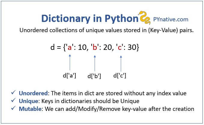
A dictionary is an unordered set of key-value pairs.
When you add a key to a dictionary, you must also add a value for that key (you can always change the value later).
Python dictionaries are optimized for retrieving the value when you know the key, but not the other way around.
Keys must be an immutable type, usually strings, but can also be tuples or numeric types.
Values can be either mutable or immutable.
# create dictionary

my_dict = { 'monday': 0, 'tuesday': 1 , 'wed': 'another day', 1:'tuesday' }
my_dict
{'monday': 0, 'tuesday': 1, 'wed': 'another day', 1: 'tuesday'}
my_dict['monday']
0
my_dict['tuesday']
1
my_dict['sda']
---------------------------------------------------------------------------
KeyError                                  Traceback (most recent call last)
<ipython-input-78-7f98da8a8c6d> in <module>
----> 1 my_dict['sda']

KeyError: 'sda'
# remove elements
del my_dict['tuesday']
my_dict
{'monday': 0, 'wed': 'another day', 1: 'tuesday'}
my_dict.keys()
dict_keys(['monday', 'wed', 1])
my_dict.values()
dict_values([0, 'another day', 'tuesday'])
my_dict.items()
dict_items([('monday', 0), ('wed', 'another day'), (1, 'tuesday')])
# updated dict_keys
my_dict['monday'] = 100
my_dict
{'monday': 100, 'wed': 'another day', 1: 'tuesday'}
Dictionaries and Booleans#
In a boolean context, an empty dictionary is false.
Any dictionary with at least one key-value pair is true.
if my_dict:
    print('it is true')

empty_dict = dict([])
if empty_dict:
    print('it is true')
it is true
Part 4: Operations, Loops, etc.#
Python’s for statement iterates over the items of any iterable sequence (e.g. a list, a tuple, a set, or a string), in the order that they appear in the sequence.
my_list = [1,2,'a','b',[3,4]]
for item in my_list:
    print(item)
1
2
a
b
[3, 4]
my_set = set([1,2,3,4,4,4])
for item in my_set:
    print(item)
1
2
3
4
The range() function#
If you do need to iterate over a sequence of numbers, the built-in function range() comes in handy. It generates arithmetic progressions:
for i in range(4):
    print(i)
0
1
2
3
for i in range(5):
    print(i)
0
1
2
3
4
# Reversed order
for i in reversed(range(6)):
    print(i)
print('---')
for item in reversed(my_list):
    print(item)
5
4
3
2
1
0
---
[3, 4]
b
a
2
1
new_list = []
for i in range(len(my_list)):
    new_list.append(my_list[-1-i])

new_list
[[3, 4], 'b', 'a', 2, 1]
my_list[::-1]
[[3, 4], 'b', 'a', 2, 1]
simple_list = list(range(10))
simple_list
[0, 1, 2, 3, 4, 5, 6, 7, 8, 9]
simple_list[0:3]
[0, 1, 2]
my_list[-1:-len(my_list)-1:-1]
[[3, 4], 'b', 'a', 2, 1]
for item in my_list[::-1]:
    print(item)
[3, 4]
b
a
2
1
Sorted order#
# random list of numbers
from random import randint
numbers = []
for __ in range(100):
    numbers.append(randint(0,1000))
randint?
Signature: randint(a, b)
Docstring:
Return random integer in range [a, b], including both end points.

File:      /usr/local/anaconda3/envs/covid/lib/python3.8/random.py
Type:      method
for item in sorted(numbers):
    print(item, end = ',')
6,11,14,14,39,42,55,86,98,118,131,136,158,168,173,198,221,221,226,246,252,255,283,302,303,304,304,308,308,320,330,342,344,346,348,350,360,372,391,447,454,463,467,473,476,483,486,489,493,509,518,522,534,551,558,579,601,622,627,634,654,660,660,662,682,684,686,693,693,695,697,712,715,727,727,735,739,777,782,804,813,818,821,824,831,839,882,901,903,903,935,939,950,953,963,968,972,973,989,995,
Enumerate function#
If you do need to iterate over a sequence of elements keeping track of the index/position of the element:
new_list = []
c = 0
for item in my_list:
    print(c, item)
    new_list.append((c,item))
    c += 1

new_list
0 1
1 2
2 a
3 b
4 [3, 4]
[(0, 1), (1, 2), (2, 'a'), (3, 'b'), (4, [3, 4])]
for x in new_list:
    c = x[0]
    item = x[1]
    print(c,item)
0 1
1 2
2 a
3 b
4 [3, 4]
x,y = (10,20)
print(x, y)
10 20
for c, item in new_list:
    print(c,item)
0 1
1 2
2 a
3 b
4 [3, 4]
strange_list = [(1,['a','b']),(2,['c','d'])]

strange_list[0]
(1, ['a', 'b'])
for i, (x,y) in strange_list:
    print(i,x,y)
1 a b
2 c d
for c, item in enumerate(my_list):
    print(c,item)
0 1
1 2
2 a
3 b
4 [3, 4]
Zip function#
We can use “zip” to loop over two or more sequences at the same time.
zip creates an iterator that aggregates elements from each of the iterables:
list_a = ['a','b','c']
list_b = [1,2,3]
list_c = ['x','y','z']

merged_list = [('a',1,'x'), ('b',2,'y'), ('c',3,'z')]
for i,j,k in zip(list_a,list_b,list_c):
    print(i,j,k)
a 1 x
b 2 y
c 3 z
zip(list_a,list_b,list_c)
<zip at 0x7fc42002e840>
list(zip(list_a,list_b,list_c))
[('a', 1, 'x'), ('b', 2, 'y'), ('c', 3, 'z')]
sources_nodes = [1,2,4,6]
target_nodes = [5,1,5,9]
weights = [3.0,2.0,1.3,3.2]

edge_list = list(zip(sources_nodes,target_nodes))
edge_list
[(1, 5), (2, 1), (4, 5), (6, 9)]
graph = {}
for source_node, target_node, weight in zip(sources_nodes,target_nodes,weights):
    graph[(source_node,target_node)] = weight
graph
{(1, 5): 3.0, (2, 1): 2.0, (4, 5): 1.3, (6, 9): 3.2}
print(edge_list,'\n')
print(list(zip(*edge_list)))
[(1, 5), (2, 1), (4, 5), (6, 9)]

[(1, 2, 4, 6), (5, 1, 5, 9)]
ss, tt = zip(*edge_list)
sources = [0,0,0,0,1,1,2,3,3,3]
targets = [1,2,3,4,4,5,6,7,8,9]
el = list(zip(sources,targets))
# what will this do?
set(list(zip(*el))[0]+list(zip(*el))[1])
{0, 1, 2, 3, 4, 5, 6, 7, 8, 9}
More on loops#
For loop#
for i in range(4):
    print(i)
0
1
2
3
While loop#
limit = 4
z = 0

while True:
    if z < limit:
        z += 1

    else:
        break
limit = 4
z = 0

while z < limit:
    print(z)
    z += 1
0
1
2
3
Break, continue, and pass statements#
The break statement#
Similar to other languages (e.g. C), this statement “breaks” out of the innermost enclosing for or while loop.
empty_list = []
for number in range(10):
    empty_list.append(number)
    if len(empty_list) > 5:
        break

print(empty_list)
[0, 1, 2, 3, 4, 5]
partial_sum = 0
i = 0
while True:
    partial_sum += numbers[i]
    i += 1
    if partial_sum > 3000:
        break

print(partial_sum)
3148
partial_sum = 0
i = 0
while partial_sum<=3000:
    partial_sum += numbers[i]
    i += 1

print(partial_sum)
3148
partial_sum = 0
while True:
    for i, number in enumerate(numbers):
        partial_sum += number
        if partial_sum > 3000:
            break
    break

print(partial_sum)
3148
The continue statement#
Also borrowed from C, this statement “continues” with the next iteration of the loop.
empty_list = []
for n in range(10):
    if n == 5:
        continue
    empty_list.append(n)

print(empty_list)
[0, 1, 2, 3, 4, 6, 7, 8, 9]
empty_list = []
for n in range(10):
    if n != 5:
        empty_list.append(n)

print(empty_list)
[0, 1, 2, 3, 4, 6, 7, 8, 9]
The pass statement#
pass does nothing. It can be used when a statement is required syntactically but the program requires no action.
# e.g. this line will yield a SyntaxError
for i in range(10):
  File "<ipython-input-126-39d65b6213c2>", line 2

    ^
SyntaxError: unexpected EOF while parsing
for i in range(10):
    pass
def some_function():
    # this should do X
    pass
Part 5: Functions#
In Python, functions:
Can return objects or not.
Can (should) have Doc Strings.
Accepts optional parameters (with defaults). If no parameter is passed, it will be equal to the default defined in the function.
Accepts parameters to be passed by name. In this case, the order in which the parameters were passed does not matter.
Have their own namespace (local scope), and therefore may obscure definitions of global scope.
Can have their properties changed (usually by decorators).
def hello():
    print("Hello, World!")
    return
hello
<function __main__.hello()>
hello()
Hello, World!
def hello(data=None):
    """
    This is a function that takes anything as `data` and returns
    a string depending on the input.

    Parameters:
    data (type): Description of the first parameter.

    Returns:
    out (str): String with the answer.
    """

    out = ''
    if data:
        out += "Hello, World!"

    else:
        out += 'Set "data" to something!'


    return out
print(hello())
print()
print(hello(x))
Set "data" to something!

Hello, World!
Making Your Functions Readable#
When you write a function, you want to be able to look at it a year from when you wrote it and still know what’s going on. There are several ways you can do this; one really helpful thing to use is a docstring.
A docstring is a long string that usually shows up right after you declare a function (so after def blah(inputs):). It should look like this, though there’s some flexibility with respect to what you do and don’t include:
def blah(inputs):
    """
    Imperative statement explaining what the function does.

    Inputs:
    input1 (type): describes the first parameter
    input2 (type): describes the second parameter
    ...

    Outputs:
    output1 (type): describes the first output
    output2 (type): describes the second output
    ...
    """
    z = some_code(inputs)
    y = do_something(z)
    # comments should be used to clarify things that look strange
    # you can also use them to label chunks of code that perform a particular operation together.

    return output1, output2
You can also indicate the types of your inputs and outputs in the function declaration, and you can set default values for the keyword arguments. Keyword arguments are optional inputs (if there is no input, the keyword argument will be set to its default value) and must appear after all required inputs are declared.
def blah1(my_number: float, my_string: str, my_bool: bool = False) -> str:
    """
    Do a string manipulation on the inputs or return a default phrase.

    Inputs:
    my_number (float): a number that is a float
    my_string (string): a string of any length
    my_bool (boolean): default False; indicates whether the default phrase will be returned

    Outputs:
    a string that is either "it was true all along!"
    or my_number and my_string concatenated into one string.
    """
    if my_bool:
        return "it was true all along!"
    else:
        return str(my_number) + ' ' + my_string

print(blah1(0.5, '0.5', True))
print(blah1(0.5, 'potatoes'))
it was true all along!
0.5 potatoes
Scope#
Recall from the very beginning of this lesson, you should also be careful about scope when writing a function. When you’re writing a function, you will have variables that are local—they only exist inside the function, and they don’t exist outside it. Other variables that you declare outside the function will not be known about in the world of the function itself. Try out this block of code, then uncomment the line that’s commented out. What happens, and why?
# Your Turn!

NUM_POTATOES = 5
print('we have this many potatoes: ', NUM_POTATOES)


def potato_peeler(words:str) -> str:
    """
    Return a string plus the phrase "but we have 4 POTATOES".

    Inputs:
    words (str): any string

    Outputs:
    (str): words plus "but we have 4 POTATOES"

    """
    # print('now we have this many potatoes: ', NUM_POTATOES)
    NUM_POTATOES = 4
    print('but now we have this many potatoes: ', NUM_POTATOES)
    return words + ' but we have ' + str(NUM_POTATOES) + ' POTATOES'


print(potato_peeler('my dog is barking'))
print('finally we have this many potatoes: ', NUM_POTATOES)
we have this many potatoes:  5
but now we have this many potatoes:  4
my dog is barking but we have 4 POTATOES
finally we have this many potatoes:  5
Part 6: NumPy#
NumPy is the fundamental package for scientific computing with Python. It contains among other things:
a powerful N-dimensional array object
sophisticated (broadcasting) functions
tools for integrating C/C++ and Fortran code
useful linear algebra, Fourier transform, and random number capabilities
Besides its obvious scientific uses, NumPy can also be used as an efficient multi-dimensional container of generic data. Arbitrary data-types can be defined. This allows NumPy to seamlessly and speedily integrate with a wide variety of databases. NumPy is licensed under the BSD license, enabling reuse with few restrictions.
Source: https://numpy.org/
NumPy for MATLAB users: https://docs.scipy.org/doc/numpy-dev/user/numpy-for-matlab-users.html
Citation: Harris, C.R., Millman, K.J., van der Walt, S.J. et al. Array programming with NumPy. Nature 585, 357–362 (2020). https://doi.org/10.1038/s41586-020-2649-2
Basic array operations#
import numpy as np
arr = np.array([0,1,2,3])
print("type of arr is:",type(arr))
arr
type of arr is: <class 'numpy.ndarray'>
array([0, 1, 2, 3])
Numpy array: Memory-efficient container that provides fast numerical operations.
L = list(range(1000))
%timeit [i**2 for i in L]
206 µs ± 1.12 µs per loop (mean ± std. dev. of 7 runs, 1000 loops each)
a = np.arange(1000)
%timeit a ** 2
626 ns ± 1.56 ns per loop (mean ± std. dev. of 7 runs, 1000000 loops each)
# array dimension and shape
a.shape
(1000,)
a.ndim
1
# 2D array
arr2d = np.array([[0,1,2],[3,4,5]])
arr2d
array([[0, 1, 2],
       [3, 4, 5]])
arr2d.ndim
2
arr2d.shape
(2, 3)
# m-D arrays
a = np.arange(5)
b = np.array([a,a])
c = np.array([b,b,b])
print(a.shape)
print(b.shape)
print(c.shape)
(5,)
(2, 5)
(3, 2, 5)
# built-in functions to create simple arrays
# evenly spaced array (similar to range in standard Python)
np.arange(10)
array([0, 1, 2, 3, 4, 5, 6, 7, 8, 9])
np.arange(1,10,0.2)
array([1. , 1.2, 1.4, 1.6, 1.8, 2. , 2.2, 2.4, 2.6, 2.8, 3. , 3.2, 3.4,
       3.6, 3.8, 4. , 4.2, 4.4, 4.6, 4.8, 5. , 5.2, 5.4, 5.6, 5.8, 6. ,
       6.2, 6.4, 6.6, 6.8, 7. , 7.2, 7.4, 7.6, 7.8, 8. , 8.2, 8.4, 8.6,
       8.8, 9. , 9.2, 9.4, 9.6, 9.8])
# linear space
np.linspace(0,1,101)
array([0.  , 0.01, 0.02, 0.03, 0.04, 0.05, 0.06, 0.07, 0.08, 0.09, 0.1 ,
       0.11, 0.12, 0.13, 0.14, 0.15, 0.16, 0.17, 0.18, 0.19, 0.2 , 0.21,
       0.22, 0.23, 0.24, 0.25, 0.26, 0.27, 0.28, 0.29, 0.3 , 0.31, 0.32,
       0.33, 0.34, 0.35, 0.36, 0.37, 0.38, 0.39, 0.4 , 0.41, 0.42, 0.43,
       0.44, 0.45, 0.46, 0.47, 0.48, 0.49, 0.5 , 0.51, 0.52, 0.53, 0.54,
       0.55, 0.56, 0.57, 0.58, 0.59, 0.6 , 0.61, 0.62, 0.63, 0.64, 0.65,
       0.66, 0.67, 0.68, 0.69, 0.7 , 0.71, 0.72, 0.73, 0.74, 0.75, 0.76,
       0.77, 0.78, 0.79, 0.8 , 0.81, 0.82, 0.83, 0.84, 0.85, 0.86, 0.87,
       0.88, 0.89, 0.9 , 0.91, 0.92, 0.93, 0.94, 0.95, 0.96, 0.97, 0.98,
       0.99, 1.  ])
np.linspace(0,1,100, endpoint = False)
array([0.  , 0.01, 0.02, 0.03, 0.04, 0.05, 0.06, 0.07, 0.08, 0.09, 0.1 ,
       0.11, 0.12, 0.13, 0.14, 0.15, 0.16, 0.17, 0.18, 0.19, 0.2 , 0.21,
       0.22, 0.23, 0.24, 0.25, 0.26, 0.27, 0.28, 0.29, 0.3 , 0.31, 0.32,
       0.33, 0.34, 0.35, 0.36, 0.37, 0.38, 0.39, 0.4 , 0.41, 0.42, 0.43,
       0.44, 0.45, 0.46, 0.47, 0.48, 0.49, 0.5 , 0.51, 0.52, 0.53, 0.54,
       0.55, 0.56, 0.57, 0.58, 0.59, 0.6 , 0.61, 0.62, 0.63, 0.64, 0.65,
       0.66, 0.67, 0.68, 0.69, 0.7 , 0.71, 0.72, 0.73, 0.74, 0.75, 0.76,
       0.77, 0.78, 0.79, 0.8 , 0.81, 0.82, 0.83, 0.84, 0.85, 0.86, 0.87,
       0.88, 0.89, 0.9 , 0.91, 0.92, 0.93, 0.94, 0.95, 0.96, 0.97, 0.98,
       0.99])
# log space
np.logspace(0,10,6, base=2)
array([1.000e+00, 4.000e+00, 1.600e+01, 6.400e+01, 2.560e+02, 1.024e+03])
np.diff(np.log10(np.logspace(0, 10, 6, base = 10)))
array([2., 2., 2., 2., 2.])
np.logspace(0, 10, 6, base = 10)
array([1.e+00, 1.e+02, 1.e+04, 1.e+06, 1.e+08, 1.e+10])
np.log10(np.logspace(0, 10, 6, base = 10))
array([ 0., 2., 4., 6., 8., 10.])
np.diff(np.log10(np.logspace(0, 10, 6, base = 10)))
array([2., 2., 2., 2., 2.])
# Common arrays
np.ones(10)
array([1., 1., 1., 1., 1., 1., 1., 1., 1., 1.])
np.ones((5,5))
array([[1., 1., 1., 1., 1.],
       [1., 1., 1., 1., 1.],
       [1., 1., 1., 1., 1.],
       [1., 1., 1., 1., 1.],
       [1., 1., 1., 1., 1.]])
np.zeros((4,4))
array([[0., 0., 0., 0.],
       [0., 0., 0., 0.],
       [0., 0., 0., 0.],
       [0., 0., 0., 0.]])
np.eye(5,5)
array([[1., 0., 0., 0., 0.],
       [0., 1., 0., 0., 0.],
       [0., 0., 1., 0., 0.],
       [0., 0., 0., 1., 0.],
       [0., 0., 0., 0., 1.]])
NumPy datatypes (examples)#
np.eye(5)
array([[1., 0., 0., 0., 0.],
       [0., 1., 0., 0., 0.],
       [0., 0., 1., 0., 0.],
       [0., 0., 0., 1., 0.],
       [0., 0., 0., 0., 1.]])
np.eye(5, dtype = int)
array([[1, 0, 0, 0, 0],
       [0, 1, 0, 0, 0],
       [0, 0, 1, 0, 0],
       [0, 0, 0, 1, 0],
       [0, 0, 0, 0, 1]])
np.eye(5, dtype = np.unicode_)
array([['1', '', '', '', ''],
       ['', '1', '', '', ''],
       ['', '', '1', '', ''],
       ['', '', '', '1', ''],
       ['', '', '', '', '1']], dtype='<U1')
Slicing and Indexing#
The items of an array can be accessed and assigned to the same way as other Python sequences (e.g. lists):
a = np.arange(100)
a
array([ 0,  1,  2,  3,  4,  5,  6,  7,  8,  9, 10, 11, 12, 13, 14, 15, 16,
       17, 18, 19, 20, 21, 22, 23, 24, 25, 26, 27, 28, 29, 30, 31, 32, 33,
       34, 35, 36, 37, 38, 39, 40, 41, 42, 43, 44, 45, 46, 47, 48, 49, 50,
       51, 52, 53, 54, 55, 56, 57, 58, 59, 60, 61, 62, 63, 64, 65, 66, 67,
       68, 69, 70, 71, 72, 73, 74, 75, 76, 77, 78, 79, 80, 81, 82, 83, 84,
       85, 86, 87, 88, 89, 90, 91, 92, 93, 94, 95, 96, 97, 98, 99])
a[1]
1
a[1:10]
array([1, 2, 3, 4, 5, 6, 7, 8, 9])
a[::-1]
array([99, 98, 97, 96, 95, 94, 93, 92, 91, 90, 89, 88, 87, 86, 85, 84, 83,
       82, 81, 80, 79, 78, 77, 76, 75, 74, 73, 72, 71, 70, 69, 68, 67, 66,
       65, 64, 63, 62, 61, 60, 59, 58, 57, 56, 55, 54, 53, 52, 51, 50, 49,
       48, 47, 46, 45, 44, 43, 42, 41, 40, 39, 38, 37, 36, 35, 34, 33, 32,
       31, 30, 29, 28, 27, 26, 25, 24, 23, 22, 21, 20, 19, 18, 17, 16, 15,
       14, 13, 12, 11, 10,  9,  8,  7,  6,  5,  4,  3,  2,  1,  0])
Illustrations of numpy array slicing and indexing

new_arr = np.arange(36).reshape((6,6))
new_arr
array([[ 0,  1,  2,  3,  4,  5],
       [ 6,  7,  8,  9, 10, 11],
       [12, 13, 14, 15, 16, 17],
       [18, 19, 20, 21, 22, 23],
       [24, 25, 26, 27, 28, 29],
       [30, 31, 32, 33, 34, 35]])
# slicing example
new_arr[4:,4:]
array([[28, 29],
       [34, 35]])
# boolean mask
new_arr[new_arr>10]
array([11, 12, 13, 14, 15, 16, 17, 18, 19, 20, 21, 22, 23, 24, 25, 26, 27,
       28, 29, 30, 31, 32, 33, 34, 35])
new_arr[[1,2],[3,4]]
array([ 9, 16])
# indexing with an array
a = np.arange(100)+10
b = np.arange(5,15)

a[b]
array([15, 16, 17, 18, 19, 20, 21, 22, 23, 24])
# notes on array copy
a = np.arange(10)
b = a[::2]
print(a)
print(b)
[0 1 2 3 4 5 6 7 8 9]
[0 2 4 6 8]
np.may_share_memory(a, b)
True
b[1] = -3
a
array([ 0, 1, -3, 3, 4, 5, 6, 7, 8, 9])
a = np.arange(10)
b = a[::2].copy()
print(a)
print(b)
[0 1 2 3 4 5 6 7 8 9]
[0 2 4 6 8]
np.may_share_memory(a, b)
False
NumPy random functions#
(Source: https://numpy.org/doc/stable/reference/random/index.html)
list_to_choose_from = [1,2,3,4,5]
print(np.random.choice(list_to_choose_from))
5
list_to_choose_from = [1,2,3,4,5,200,300,23,22]
for _ in range(5):
    print(np.random.choice(list_to_choose_from))
2
200
4
2
22
list_to_choose_from = [1,2,3,4,5,200,300,23,22,0]
probs = [0.91]+[0.01]*(len(list_to_choose_from)-1)
for _ in range(5):
    print(np.random.choice(list_to_choose_from, p=probs))
1
1
1
1
1
list_to_choose_from = [1,2,3,4,5]
print("replace=False:",np.random.choice(list_to_choose_from, size=5, replace=False))

list_to_choose_from = [1,2,3,4,5]
print("replace=True:",np.random.choice(list_to_choose_from, size=5, replace=True))
replace=False: [4 3 1 2 5]
replace=True: [1 5 1 1 5]
np.random.randint(0,2,size=100)
array([1, 0, 0, 0, 1, 1, 1, 0, 0, 1, 1, 0, 0, 1, 0, 0, 0, 1, 0, 0, 0, 1,
       0, 0, 1, 1, 1, 0, 1, 1, 0, 1, 0, 1, 0, 0, 1, 1, 0, 0, 0, 1, 0, 1,
       0, 1, 1, 0, 1, 0, 1, 1, 1, 1, 0, 0, 0, 1, 1, 1, 0, 0, 0, 1, 0, 1,
       0, 1, 1, 0, 0, 1, 1, 0, 0, 0, 1, 1, 0, 1, 0, 0, 1, 1, 0, 0, 1, 0,
       1, 0, 1, 0, 1, 0, 1, 0, 0, 0, 0, 0])
np.random.randint(0,200,size=(5,5))
array([[ 60, 160, 182, 103,  28],
       [ 66,  25,  70, 191,  57],
       [160, 157,  36, 194,  49],
       [ 89,  46,  27, 112, 129],
       [148, 136, 129, 162,  98]])
np.random.normal(0,1,size=20)
array([ 1.38538459, -0.22499655,  0.44265991,  1.84486781,  0.91635511,
       -1.49724389, -1.56061478,  0.40359774, -0.22923305,  1.26643928,
        0.6307696 , -0.30890966, -0.39230262,  0.06575317, -0.10915068,
        1.01247965, -0.56251802, -0.8125841 ,  1.9370336 ,  1.75435461])
probs = [0.9]+[0.01]*10

np.random.multinomial(100, pvals=probs)
array([90, 0, 1, 0, 2, 1, 0, 1, 2, 2, 1])
np.random.multinomial(100, pvals=probs, size=5)
array([[92,  0,  0,  1,  1,  0,  0,  4,  1,  0,  1],
       [91,  0,  1,  1,  1,  1,  1,  1,  1,  1,  1],
       [86,  0,  0,  0,  3,  0,  0,  6,  1,  2,  2],
       [90,  2,  1,  1,  0,  2,  2,  0,  1,  0,  1],
       [92,  2,  3,  1,  0,  0,  1,  0,  0,  1,  0]])
A = np.random.randint(1,6,size=(3,3))
A
array([[2, 2, 3],
       [1, 1, 5],
       [1, 4, 5]])
NumPy Arithmetics, etc.#
np.sum(A)
24
A.sum(axis = 0)
array([ 4, 7, 13])
A.sum(axis = 1)
array([ 7, 7, 10])
A.T
array([[2, 1, 1],
       [2, 1, 4],
       [3, 5, 5]])
A.transpose()
array([[2, 1, 1],
       [2, 1, 4],
       [3, 5, 5]])
A.reshape(9)
array([2, 2, 3, 1, 1, 5, 1, 4, 5])
A.reshape(9).reshape((3,3))
array([[2, 2, 3],
       [1, 1, 5],
       [1, 4, 5]])
A.reshape(9).reshape((3,3)).reshape(-1)
array([2, 2, 3, 1, 1, 5, 1, 4, 5])
A.flatten()
array([2, 2, 3, 1, 1, 5, 1, 4, 5])
np.log(A)
array([[0.69314718, 0.69314718, 1.09861229],
       [0.        , 0.        , 1.60943791],
       [0.        , 1.38629436, 1.60943791]])
np.log10(A)
array([[0.30103   , 0.30103   , 0.47712125],
       [0.        , 0.        , 0.69897   ],
       [0.        , 0.60205999, 0.69897   ]])
np.sqrt(A)
array([[1.41421356, 1.41421356, 1.73205081],
       [1.        , 1.        , 2.23606798],
       [1.        , 2.        , 2.23606798]])
np.power(A,2)
array([[ 4,  4,  9],
       [ 1,  1, 25],
       [ 1, 16, 25]])
A
array([[2, 2, 3],
       [1, 1, 5],
       [1, 4, 5]])
A*A
array([[ 4,  4,  9],
       [ 1,  1, 25],
       [ 1, 16, 25]])
A@A
array([[ 9, 18, 31],
       [ 8, 23, 33],
       [11, 26, 48]])
A.dot(A)
array([[ 9, 18, 31],
       [ 8, 23, 33],
       [11, 26, 48]])
np.dot(A,A)
array([[ 9, 18, 31],
       [ 8, 23, 33],
       [11, 26, 48]])
np.vstack([A,A])
array([[2, 2, 3],
       [1, 1, 5],
       [1, 4, 5],
       [2, 2, 3],
       [1, 1, 5],
       [1, 4, 5]])
np.hstack([A,A])
array([[2, 2, 3, 2, 2, 3],
       [1, 1, 5, 1, 1, 5],
       [1, 4, 5, 1, 4, 5]])
A
array([[2, 2, 3],
       [1, 1, 5],
       [1, 4, 5]])
np.diag(A)
array([2, 1, 5])
np.diag([1,2,3])
array([[1, 0, 0],
       [0, 2, 0],
       [0, 0, 3]])
np.unique(A)
array([1, 2, 3, 4, 5])
Part 7: Matplotlib#
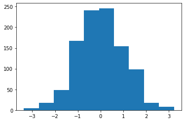
import matplotlib.pyplot as plt
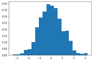
npoints = 1000
data = np.random.normal(0,1,npoints)
plt.hist(data);
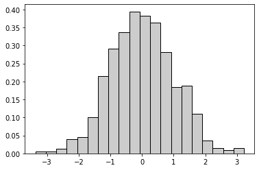
plt.hist(data,bins=20,density=True);
plt.hist(data,bins=20,lw=1,ec='k',fc='.8',density=True);
Matplotlib Tip 1:#
Problem: “I never remember which matplotlib functions have “set_” in front of them and which dont… also how do you make log-scaled axes? Also ughhh.”
Solution: Commit to making everything a subplot.
w = 4
h = 3
fig, ax = plt.subplots(1, 1, figsize=(w,h), dpi=150)


plt.show()
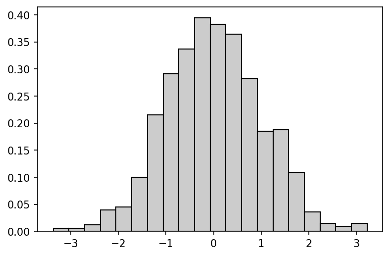
w = 6.0
h = 4.0
fig, ax = plt.subplots(1, 1, figsize=(w,h), dpi=150)

# note the "ax" instead of the "plt"!
ax.hist(data,bins=20,lw=1,ec='k',fc='.8',density=True)

plt.show()
w = 6.0
h = 4.0
fig, ax = plt.subplots(1, 1, figsize=(w,h), dpi=150)
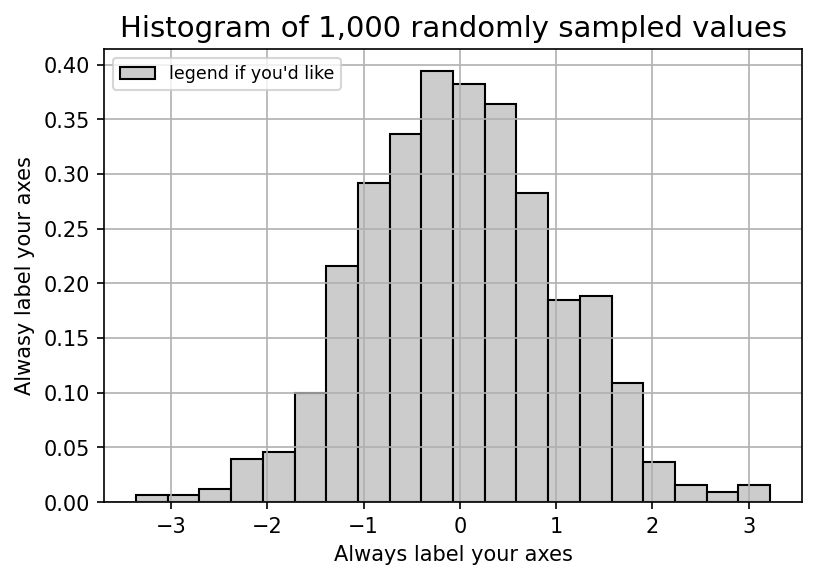
data_label = "legend if you'd like"
ax.hist(data,bins=20,lw=1,ec='k',fc='.8',density=True,label=data_label)
ax.legend(loc=2,fontsize='small')
ax.set_title('Histogram of 1,000 randomly sampled values',fontsize=14)
ax.set_xlabel('Always label your axes')
ax.set_ylabel('Alwasy label your axes')
## uncomment below to get the grid's default placement to be behind the bars
# from matplotlib import rc
# rc('axes', axisbelow=True)
ax.grid()
plt.show()
Matplotlib Tip 2:#
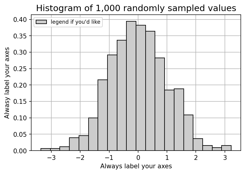
Think about future you. You might be sharing these figs with colleagues. In that case, a simple png is nice. Same with slides. If you’re putting them into your manuscript, 97% of the time, you’re gonna wanna use pdfs.
I usually have a directory structure that looks something like:
code/
this_notebook.ipynb
other_dot_py_files.py
data/
figs/
pngs/
figure1.png
etc…
pdfs/
figure1.pdf
etc…
# uncomment below to get the grid's default placement to be behind the bars
from matplotlib import rc
rc('axes', axisbelow=True)

# uncomment below if you want the output images to have a white (as opposed to transparent) background
rc('axes', fc='w')
rc('figure', fc='w')
rc('savefig', fc='w')
w = 6.0
h = 4.0
fig, ax = plt.subplots(1, 1, figsize=(w,h), dpi=150)

data_label = "legend if you'd like"
ax.hist(data,bins=20,lw=1,ec='k',fc='.8',density=True,label=data_label)

ax.legend(loc=2,fontsize='small')
ax.set_title('Histogram of 1,000 randomly sampled values',fontsize=14)
ax.set_xlabel('Always label your axes')
ax.set_ylabel('Alwasy label your axes')

ax.grid()

plt.savefig('images/pngs/class_01_figure1.png', dpi=425, bbox_inches='tight')
plt.savefig('images/pdfs/class_01_figure1.pdf', bbox_inches='tight')

plt.show()
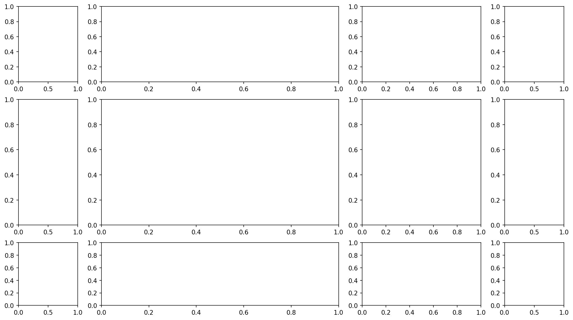
Matplotlib Tip 3#
Different SIZED subplOTS
w = 4
h = 3
nrows = 3
ncols = 4
fig, ax = plt.subplots(nrows, ncols, figsize=(w*ncols,h*nrows), dpi=150,
                       gridspec_kw={"width_ratios": [0.5, 2.0, 1.0, 0.5],
                                    "height_ratios":[0.6, 1.0, 0.5]})

plt.show()
w = 4
h = 3
nrows = np.random.randint(6)+2
ncols = np.random.randint(6)+2
fig, ax = plt.subplots(nrows, ncols, figsize=(w*ncols,h*nrows), dpi=150,
                       gridspec_kw={"width_ratios": np.random.uniform(0.1, 1.5, ncols),
                                    "height_ratios":np.random.uniform(0.1, 1.5, nrows)})

plt.show()
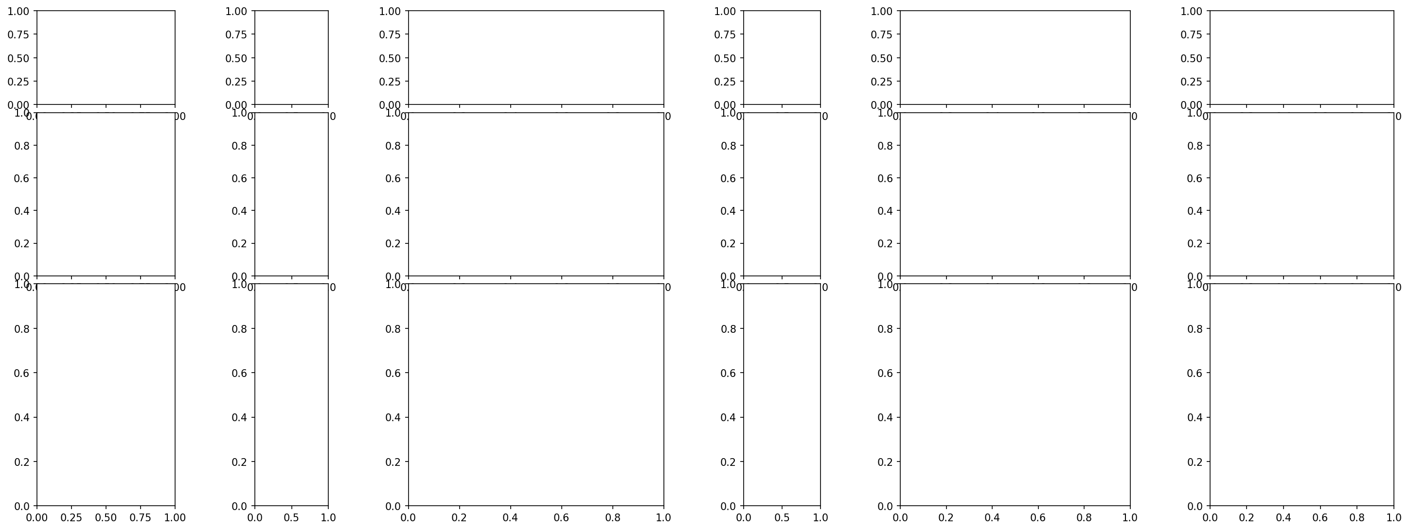
Matplotlib Tip 4#
Spacing! Between! __ - _ _ - _ Your! _ _ _ Subplots
w = 4
h = 3
nrows = np.random.randint(6)+2
ncols = np.random.randint(6)+2
fig, ax = plt.subplots(nrows, ncols, figsize=(w*ncols,h*nrows), dpi=150,
gridspec_kw={"width_ratios": np.random.uniform(0.1, 1.5, ncols),
"height_ratios":np.random.uniform(0.1, 1.5, nrows)})
plt.subplots_adjust(wspace=0.50, hspace=0.05)
# not that much "heightspace" between subplots, kinda a lot of "widthspace"
plt.show()
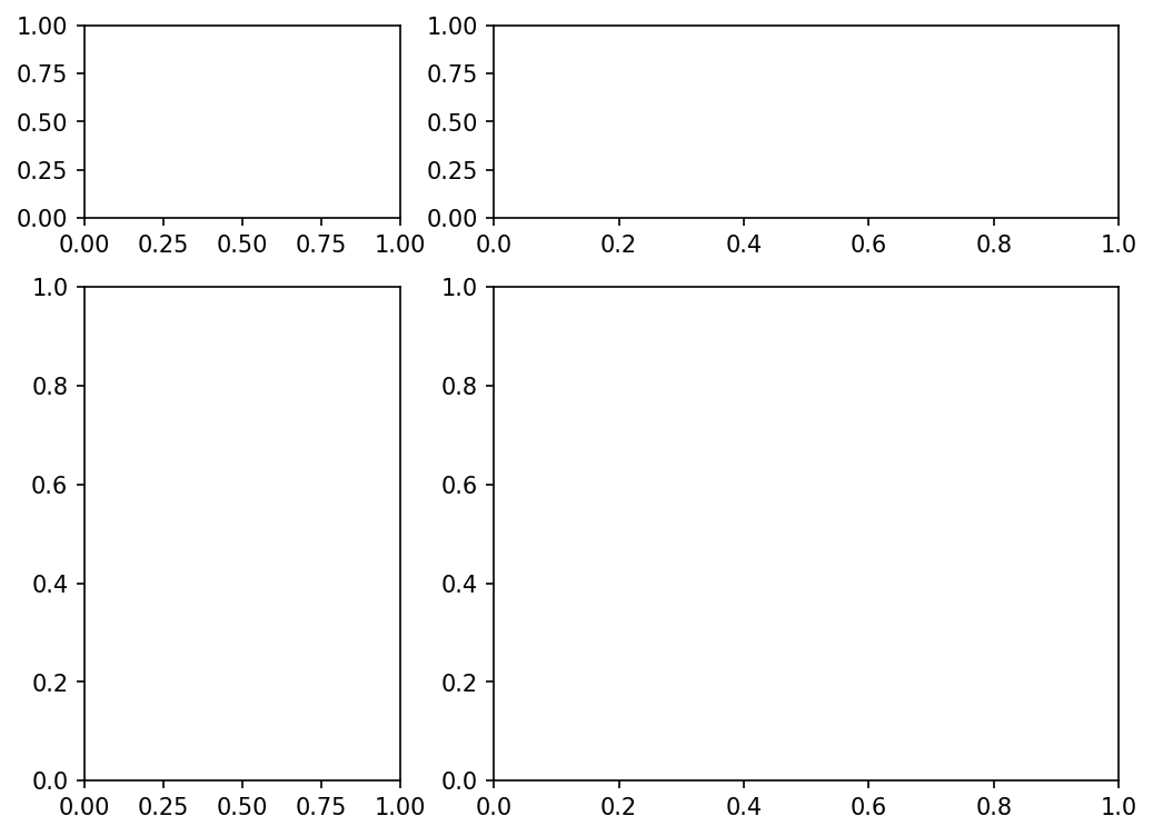
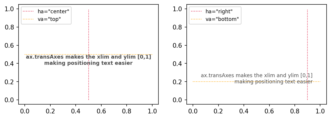
Matplotlib Tip 5:#
Text! Place it great!
There are two ways / ideaologies about how to place text on a subplot.
My text is being placed in a specific spot on the subplot and all I need to know is coordinates between 0 and 1
My text is data-relevant and as such I need my xpos and ypos to have the same domain as my data
w = 4.5
h = 3
ncols = 2
nrows = 1
fig, ax = plt.subplots(nrows, ncols, figsize=(w*ncols,h*nrows), dpi=150)
actualtext = 'ax.transAxes makes the xlim and ylim [0,1]\nmaking positioning text easier'
############ ax[0]
xpos0 = 0.5
ypos0 = 0.5
ax[0].text(xpos0, ypos0, actualtext, transform=ax[0].transAxes,
ha='center', va='top', color='.3', fontsize='small', fontweight='bold')
ax[0].vlines(xpos0, 0, 1, linestyle=':', linewidth=1, color='crimson', label='ha="center"')
ax[0].hlines(ypos0, 0, 1, linestyle=':', linewidth=1, color='orange', label='va="top"')
ax[0].legend(fontsize='small', loc=2)
############ ax[1]
xpos1 = 0.9
ypos1 = 0.2
ax[1].text(xpos1, ypos1, actualtext, transform=ax[1].transAxes,
ha='right', va='bottom', color='.3', fontsize='small')
ax[1].vlines(xpos1, 0, 1, linestyle=':', linewidth=1, color='crimson', label='ha="right"')
ax[1].hlines(ypos1, 0, 1, linestyle=':', linewidth=1, color='orange', label='va="bottom"')
ax[1].legend(fontsize='small', loc=2)
plt.savefig('images/pngs/class_01_figure2.png', dpi=425, bbox_inches='tight')
plt.savefig('images/pdfs/class_01_figure2.pdf', bbox_inches='tight')
plt.show()
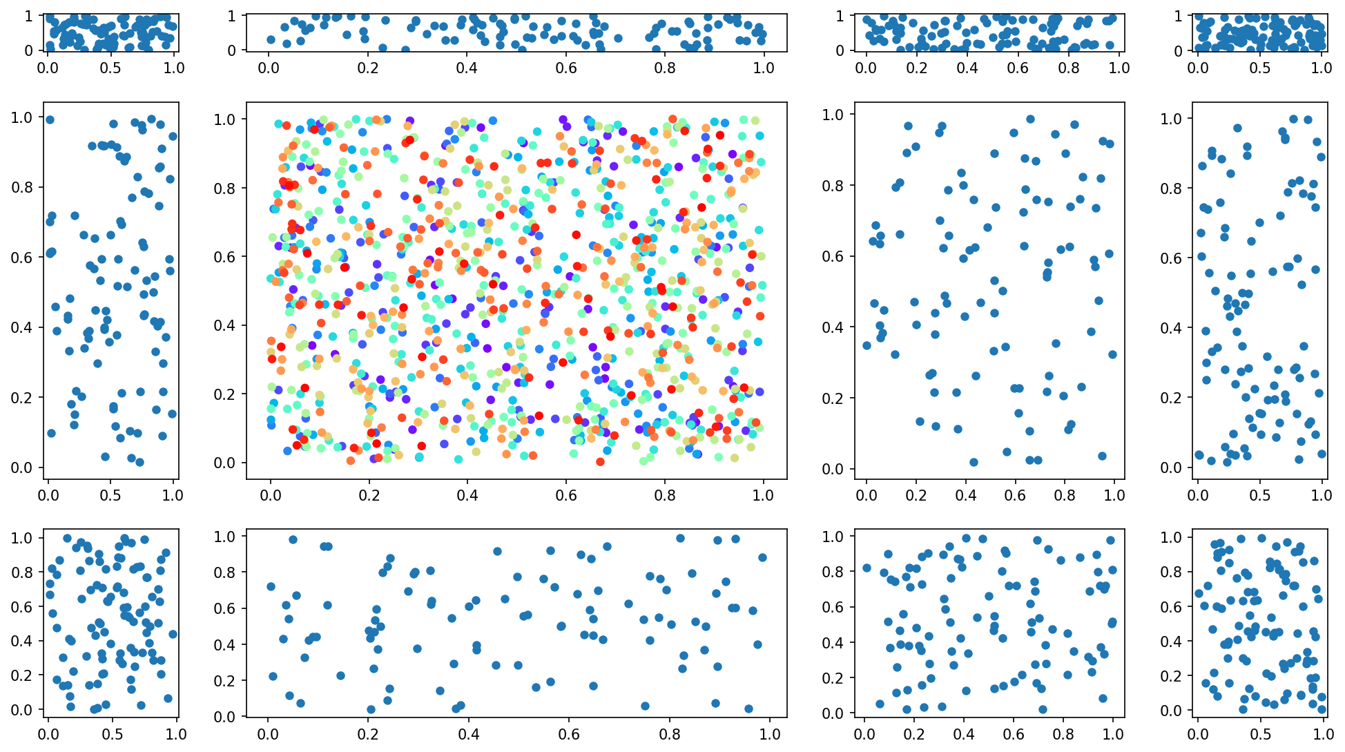
Matplotlib Tip 6:#
itertools is your friend and likely your best friend. Check this out for getting the list of your axis tuples
import itertools as it
w = 4
h = 3
nrows = 3
ncols = 4
fig, ax = plt.subplots(nrows, ncols, figsize=(w*ncols,h*nrows), dpi=150,
gridspec_kw={"width_ratios": [0.5, 2.0, 1.0, 0.5],
"height_ratios":[0.1, 1.0, 0.5]})
plt.subplots_adjust(wspace=0.25, hspace=0.25)
####*****####
tups = list(it.product(range(nrows), range(ncols)))
print("These are all your axis indices:",tups)
####*****####
for i, tup in enumerate(tups):
if tup != (1,1):
ax[tup].scatter(np.random.uniform(0,1,100),np.random.uniform(0,1,100), lw=0)
else:
ax[tup].scatter(np.random.uniform(0,1,1000),np.random.uniform(0,1,1000),
c=np.linspace(0,1,1000), cmap='rainbow', lw=0)
plt.savefig('images/pngs/class_01_figure3.png', dpi=425, bbox_inches='tight')
plt.savefig('images/pdfs/class_01_figure3.pdf', bbox_inches='tight')
plt.show()
These are all your axis indices: [(0, 0), (0, 1), (0, 2), (0, 3), (1, 0), (1, 1), (1, 2), (1, 3), (2, 0), (2, 1), (2, 2), (2, 3)]
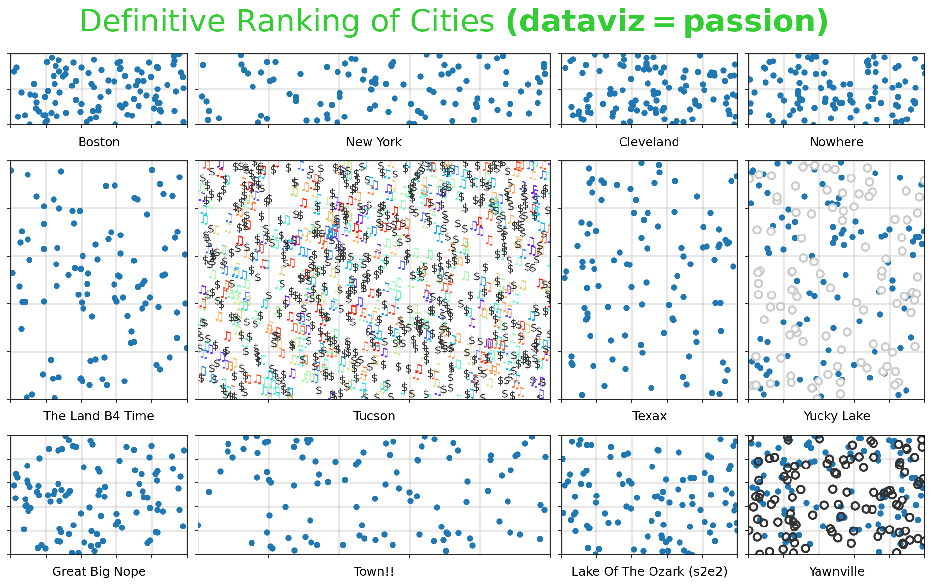
Matplotlib Tip 7:#
do something to all the subplots.
Highly encouraged to make that something be adding grids
import warnings
warnings.filterwarnings("ignore", category=UserWarning)
w = 4
h = 3
nrows = 3
ncols = 4
fig, ax = plt.subplots(nrows, ncols, figsize=(w*ncols,h*nrows), dpi=150,
gridspec_kw={"width_ratios": [1.0, 2.0, 1.0, 1.0],
"height_ratios":[0.3, 1.0, 0.5]})
plt.subplots_adjust(wspace=0.05, hspace=0.25)
tups = list(it.product(range(nrows), range(ncols)))
for i, tup in enumerate(tups):
if tup != (1,1):
ax[tup].scatter(np.random.uniform(0,1,100),np.random.uniform(0,1,100), lw=0)
else:
ax[tup].scatter(np.random.uniform(0,1,500),np.random.uniform(0,1,500),
c=np.linspace(0,1,500), cmap='rainbow', lw=0, marker="$\u266B$", s=100)
ax[tup].scatter(np.random.uniform(0,1,500),np.random.uniform(0,1,500),
c='.2', lw=0, marker="$\$$", s=100)
if tup == (2,3):
ax[tup].scatter(np.random.uniform(0,1,100),np.random.uniform(0,1,100),
lw=2, c='None', ec='.2', s=50)
if tup == (1,3):
ax[tup].scatter(np.random.uniform(0,1,100),np.random.uniform(0,1,100),
lw=2, c='w', ec='.8', s=50)
xlabs = ['Boston', 'New York', 'Cleveland', 'Nowhere', 'The Land B4 Time', 'Tucson',
'Texax', 'Yucky Lake', 'Great Big Nope', 'Town!!', 'Lake Of The Ozark (s2e2)', 'Yawnville']
plt.suptitle(r'Definitive Ranking of Cities $\mathbf{(dataviz=passion)}$', y=0.95, fontsize=30, color='limegreen')
for ai, a in enumerate(fig.axes):
a.grid(linewidth=2, alpha=0.3, color='0.7')
a.set_xlabel(xlabs[ai], fontsize='large')
a.set_xlim(0,1)
a.set_ylim(0,1)
a.set_xticklabels(["" for i in a.get_xticks()])
a.set_yticklabels(["" for i in a.get_yticks()])
plt.savefig('images/pngs/class_01_figure4.png', dpi=425, bbox_inches='tight')
plt.savefig('images/pdfs/class_01_figure4.pdf', bbox_inches='tight')
plt.show()
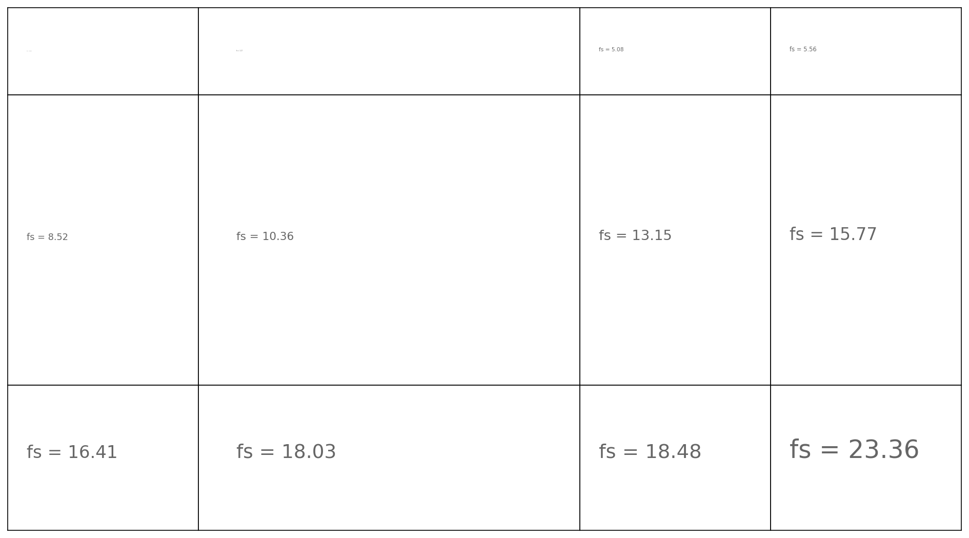
Matplotlib Tip 8:#
Writing a paper? How about one baseline fontsize?
also sneaking a “set_xticks([])” into this one
fs = 12
w = 4
h = 3
nrows = 3
ncols = 4
fig, ax = plt.subplots(nrows, ncols, figsize=(w*ncols,h*nrows), dpi=150,
gridspec_kw={"width_ratios": [1.0, 2.0, 1.0, 1.0],
"height_ratios":[0.3, 1.0, 0.5]})
plt.subplots_adjust(wspace=0.0, hspace=0.0)
tups = list(it.product(range(nrows), range(ncols)))
for ai, tup in enumerate(tups):
fs_i = fs * (2*ai/len(tups)) + np.random.uniform(-2,2)
ax[tup].text(0.1, 0.5, 'fs = %.2f'%fs_i, fontsize=fs_i, color='.4', ha='left')
ax[tup].set_xticks([])
ax[tup].set_yticks([])
plt.savefig('images/pngs/class_01_figure5.png', dpi=425, bbox_inches='tight')
plt.savefig('images/pdfs/class_01_figure5.pdf', bbox_inches='tight')
plt.show()
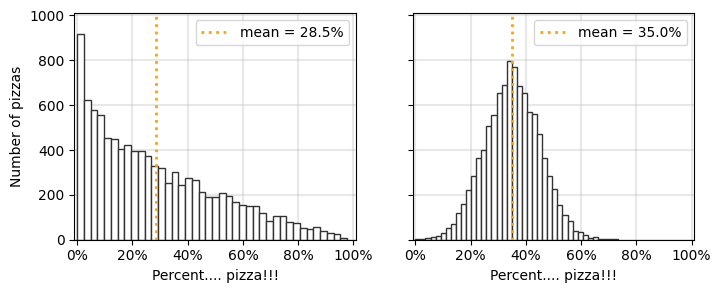
Matplotlib Tip 9:#
Here’s a small one, how about putting percentages instead of fractions?
Also sneaking a sharey=True into this tip
from matplotlib import ticker
raw_data1 = np.random.beta(0.8, 2, 10000)
raw_data1[raw_data1<=0] = 0
raw_data2 = np.random.normal(0.35, 0.1, 10000)
raw_data2[raw_data2<=0] = 0
fs = 12
w = 4
h = 3
nrows = 1
ncols = 2
fig, ax = plt.subplots(nrows, ncols, figsize=(w*ncols,h*nrows), dpi=100, sharey=True)
ax[0].hist(raw_data1, bins=40, ec='.2', color='w')
yticks = ax[0].get_yticks()
ax[0].vlines(np.mean(raw_data1), 0, yticks[-1]*1.01, color='orange',
label='mean = %.1f%%'%(np.mean(raw_data1)*100), linestyle=':', lw=2)
ax[1].hist(raw_data2, bins=40, ec='.2', color='w')
ax[1].vlines(np.mean(raw_data2), 0, yticks[-1]*1.01, color='orange',
label='mean = %.1f%%'%(np.mean(raw_data2)*100), linestyle=':', lw=2)
ax[0].set_ylabel('Number of pizzas')
for a in fig.axes:
a.xaxis.set_major_formatter(ticker.PercentFormatter(xmax=1.0))
a.set_xlim(-0.01,1.01)
a.set_ylim(yticks[0], yticks[-1]*1.01)
a.legend()
a.grid(linewidth=1.5, color='.7', alpha=0.3)
a.set_xlabel('Percent.... pizza!!!')
plt.savefig('images/pngs/class_01_figure6.png', dpi=425, bbox_inches='tight')
plt.savefig('images/pdfs/class_01_figure6.pdf', bbox_inches='tight')
plt.show()
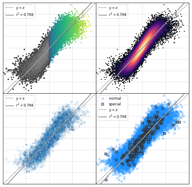
Matplotlib Tip 10:#
(worried whisper…)
…It’s scatterplot week….
(pronounced like a Great British Bakeoff contestant)
from scipy.stats import gaussian_kde
from scipy.stats import linregress
# so let's play with some fake data
raw_data_x = np.array(sorted(np.random.normal(0.5,0.25,20000)))
raw_data_y = np.linspace(0.01,0.99,20000)+np.random.normal(0.0,0.125,20000)
slope, intercept, rvalue, pvalue, stderr = linregress(raw_data_x, raw_data_y)
xslope = [min(raw_data_x), max(raw_data_x)]
yslope = [xslope[i]*slope+intercept for i in range(len(xslope))]
w = 4
h = 4
nrows = 2
ncols = 2
fig, ax = plt.subplots(nrows, ncols, figsize=(w*ncols,h*nrows), dpi=100)
plt.subplots_adjust(hspace=0,wspace=0)
tups = list(it.product(range(nrows), range(ncols)))
########## ax[(0,0)]
ax[tups[0]].scatter(raw_data_x[:10000], raw_data_y[:10000], ec='w',
lw=0.1, s=np.random.normal(12,2.5,10000), c='.2')
ax[tups[0]].scatter(raw_data_x[10000:], raw_data_y[10000:], ec='w',
lw=0, s=10, c=raw_data_x[::2], cmap='viridis', alpha=0.9)
########## ax[(0,1)]
xy = np.vstack([raw_data_x, raw_data_y])
z = gaussian_kde(xy)(xy)
ax[tups[1]].scatter(raw_data_x, raw_data_y, lw=0, s=5, c=z, cmap='magma', alpha=0.9, marker='s')
########## ax[(1,0)]
cc = plt.cm.Blues(np.random.uniform(0.3,1,len(raw_data_x)))
ax[tups[2]].scatter(raw_data_x, raw_data_y, lw=np.random.beta(0.2, 2.0, len(raw_data_x)),
s=np.random.uniform(2, 30, len(raw_data_x)), fc='None', ec=cc, marker='o')
########## ax[(1,1)]
inds = np.random.choice(range(len(raw_data_x)), size=int(0.01*len(raw_data_x)), replace=False)
ax[tups[3]].scatter(raw_data_x, raw_data_y, lw=0, s=40, c='dodgerblue',
marker='X', alpha=0.35, label='normal')
ax[tups[3]].scatter(raw_data_x[inds], raw_data_y[inds], lw=1, s=40, c='None',
marker='X', ec='.2', label='special')
for a in fig.axes:
a.set_ylim(-0.5,1.5)
a.set_xlim(-0.5,1.5)
a.plot([-2,2],[-2,2],color='.3',linestyle=':',label=r'$y=x$')
a.plot(xslope, yslope, color='.6', linewidth=2, label=r'$r^2 = %.3f$'%(rvalue**2))
a.grid(linewidth=1.25, color='.7', alpha=0.3)
a.set_xticklabels(["" for i in a.get_xticks()])
a.set_yticklabels(["" for i in a.get_xticks()])
a.tick_params(axis='both',which='both',length=0)
a.legend(loc=2, fontsize='small')
plt.savefig('images/pngs/class_01_figure7.png', dpi=425, bbox_inches='tight')
plt.savefig('images/pdfs/class_01_figure7.pdf', bbox_inches='tight')
plt.show()
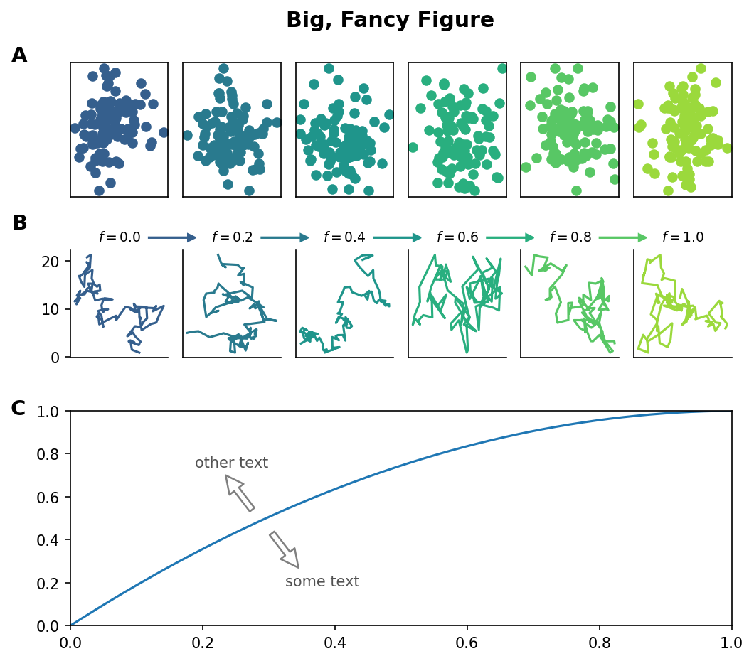
Matplotlib Tip 11:#
Spanning subplots for dramatic multi-panel figures
import matplotlib.pyplot as plt
import numpy as np
import matplotlib
from matplotlib import gridspec
# Set figure params
nrows = 3 # number of rows in the plot
ncols = 6 # number of columns
cols = plt.cm.viridis(np.linspace(0.3,0.85,ncols))
fs = np.round(np.linspace(0,1,ncols),2)
# First define the figure environment
plt.figure(dpi=150, figsize=(8,7))
# Next, define the "GridSpec"
gs = gridspec.GridSpec(nrows,
ncols,
width_ratios=[1]*ncols,
height_ratios=[1.25, 1, 2])
# Now, plot the data
for i in range(ncols):
f = fs[i]
##### TOP ROW ######
ax_row1_i = plt.subplot(gs[i])
xvs = np.random.normal(0,1,100)
yvs = np.random.normal(0,1,100)
ax_row1_i.scatter(xvs,yvs,color=cols[i])
ax_row1_i.set_xticks([])
ax_row1_i.set_yticks([])
####################
##### SECOND ROW ######
ax_row2_i = plt.subplot(gs[i+ncols])
ax_row2_i.plot(np.cumsum(xvs),
np.cumsum(yvs),color=cols[i])
if i!=ncols-1:
ax_row2_i.arrow(0.8, 1.115, 0.4, 0, head_width=0.07, head_length=0.08, width=0.008,
fc=cols[i], ec=cols[i],transform=ax_row2_i.transAxes,clip_on=False)
if i > 0:
ax_row2_i.set_yticks([])
else:
ax_row1_i.text(-0.60, 1.05,'A',
fontsize=14,
transform=ax_row1_i.transAxes,
fontweight='semibold',
va='center',
ha='left',clip_on=False)
ax_row2_i.text(-0.60, 1.25,'B',
fontsize=14,
transform=ax_row2_i.transAxes,
fontweight='semibold',
va='center',
ha='left',clip_on=False)
ax_row2_i.spines['top'].set_visible(False)
ax_row2_i.spines['right'].set_visible(False)
ax_row2_i.set_xticks([])
ax_row2_i.set_title('$f = %.1f$'%f, fontsize=9,y=1)
#######################
######## BOTTOM ROW #########
axi = plt.subplot(gs[nrows-1,:]) # this makes the subplot span axes
xvals = np.linspace(0,1)
axi.plot(xvals,1-(np.cumsum(xvals)/sum(xvals))[::-1])
axi.annotate("",
xy=(0.23, 0.72),
xytext=(0.28, 0.52),
transform=axi.transAxes,
arrowprops=dict(shrink=0.1, ec='#808080',fc='w',lw=1.2))
axi.text(0.30, 0.725,
'other text',
fontsize=10,
transform=axi.transAxes,
color='#525252',
va='bottom',ha='right')
axi.annotate("",
xy=(0.35, 0.25),
xytext=(0.30, 0.45),
transform=axi.transAxes,
arrowprops=dict(shrink=0.1, ec='#808080',fc='w',lw=1.2))
axi.text(0.325, 0.2375,
'some text',
fontsize=10,
transform=axi.transAxes,
color='#525252',
va='top',ha='left')
axi.set_xlim(0,1)
axi.set_ylim(0,1)
axi.text(-0.09, 1.01,'C',
fontsize=14,
transform=axi.transAxes,
fontweight='semibold',
va='center',
ha='left',clip_on=False)
#############################
plt.suptitle('Big, Fancy Figure',y=0.95,fontweight='semibold',fontsize='x-large')
plt.subplots_adjust(wspace=0.15, hspace=0.35)
plt.savefig('images/pngs/class_01_figure8.png', dpi=425, bbox_inches='tight')
plt.savefig('images/pdfs/class_01_figure8.pdf', bbox_inches='tight')
plt.show()
Can you think of any more great tips for making visualizations in matplotilb? Send them our way!
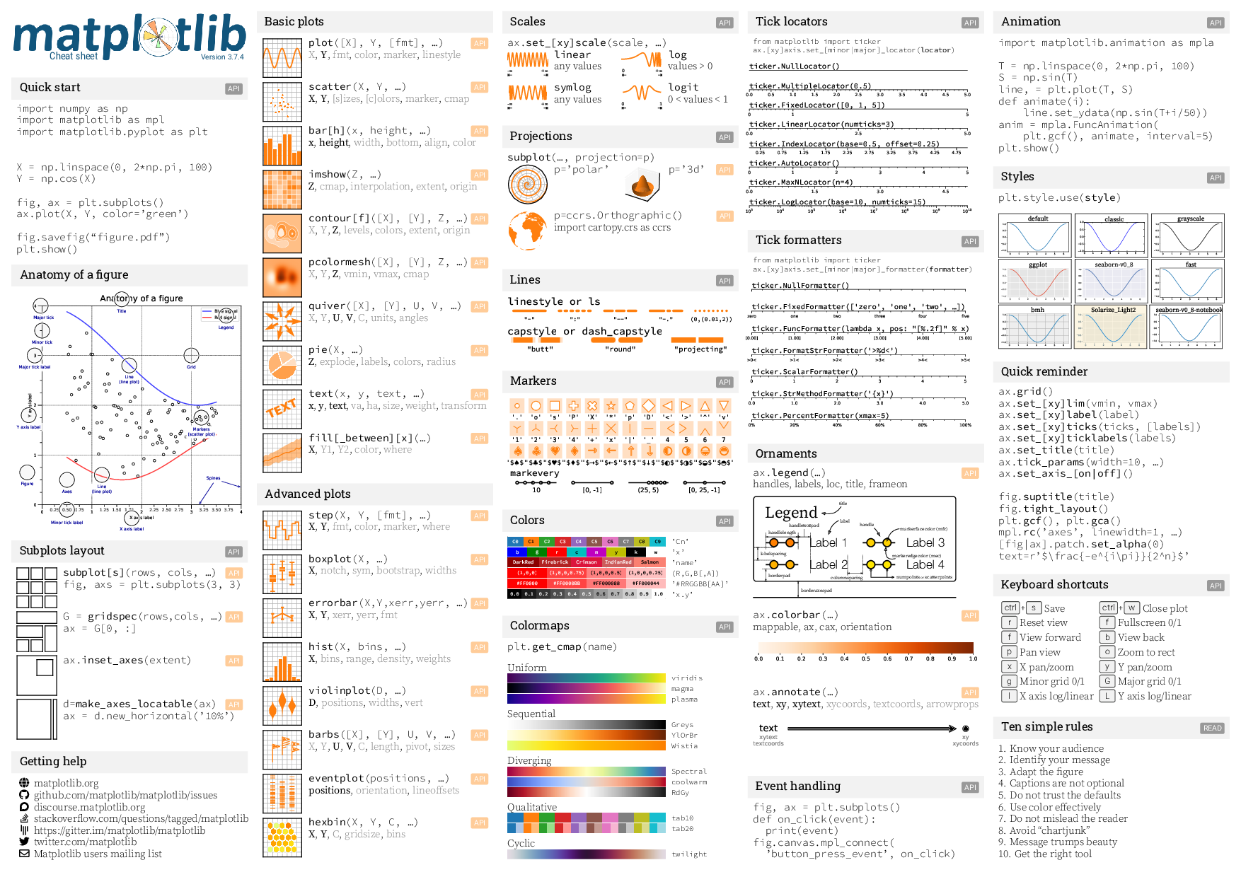
Matplotlib Cheatsheet#
Next time…#
Networks and networkx! class_02_networkx1.ipynb
References and further resources:#
Class Webpages
Jupyter Book: https://asmithh.github.io/network-science-data-book/intro.html
Syllabus and course details: https://brennanklein.com/phys7332-fall24
Data Visualization with matplotlib: https://matplotlib.org/stable/plot_types/index.html
Intro Python & Numpy: https://numpy.org/numpy-tutorials/
Harris, C.R., Millman, K.J., van der Walt, S.J. et al. Array programming with NumPy. Nature 585, 357–362 (2020). https://doi.org/10.1038/s41586-020-2649-2