Class 15: Machine Learning 2 — Building up to Graph Convolutional Networks#
Today’s Goals#
Think about how graph neural networks operate at a high level.
Understand what the building blocks of a graph neural network are.
Play with a graph neural network’s hyperparameters.
Backpropagation (by request):#
At a very high level, backpropagation is how we adjust our weights, going back from the output layer (and our loss function) all the way back to the weights from the input layer.
It involves computing a bunch of partial derivatives (gradients) and adjusting our weights/biases (the parameters we’re learning in our neural network) according to the relationship between the gradients and the loss.
What ingredients do we need to do backpropagation?#
First, we need a loss function. Our loss function (or cost function) needs to be differentiable with respect to the weights and biases we use in the network. Our loss also has to be expressed as a function of the input and our weights and biases. For example, let’s look at a toy example with one hidden layer and a mean squared error (MSE) loss function.
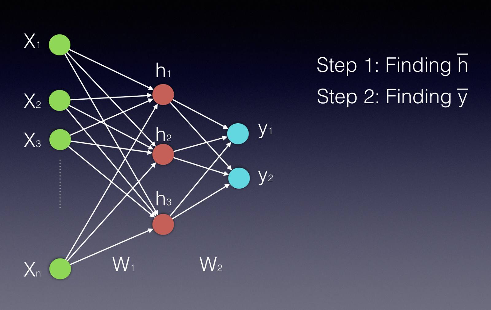
The simplified output \(g(\vec{x}) of our neural network with input \)\vec{x}\(, given weight matrices \)W^{(1)}\( and \)W^{(2)}\( and generic activation functions \)\sigma^{(1)}\( and \)\sigma^{(2)}$, is
Our loss function, with ground truth \(\vec{z}\), is \(\lvert \lvert g(\vec{x}) - \vec{z} \rvert \rvert\). In the generalized sense, we can use a generic loss function \(C(g(\vec{x}), \vec{z})\).
Next, we need partial derivatives and the chain rule!
This is how backpropagation adjusts the weights – we compute the partial derivative of our cost function \(C\) with respect to one weight from node \(i\) to node \(j\) in the \(2^{nd}\) matrix of weights:
Here, \(y_j\) is the \(j^{th}\) output of our network (in the output layer).
In other words, we’re passing the dot product of row \(j\) of \(W^{(2)}\) and \(\vec{h}\), our hidden layer’s output, through a sigmoid function. Let’s call \(\sum_{i}w^{(2)}_{ij} * h_i\) \(o_j\), and let’s expand our partial derivative expression using the chain rule once more.
What are we doing here? We’re tracing how our specific weight \(w^{(2)}_{ij}\) affects our computed loss for a particular input (or batch of inputs).
We know that \(\frac{\delta y_j}{o_j}\) is the partial derivative of the activation function \(\sigma^{(2)}\).
Additionally, we know that \(\frac{o_j}{\delta w^{(2)}_{ij}}\) is
Only one term in this sum relies on \(w^{(2)}_{ij}\) – that’s \(w^{(2)}_{ij} h_i\). This means this part of our partial derivative reduces to
Now let’s look at \(\frac{\delta y_j}{h_j}\). Let’s say we’re using a sigmoid activation function; in this case, this part of our partial derivative is
If we’re using MSE for the loss function \(C\) and \(\vec{z}\) is our ground truth answer,
$\(\frac{\delta C}{\delta y_j} = 2 (z_j - y_j)\)$.
Therefore, the gradient of our loss with respect to \(w^{(2)}_{ij}\) is
$\(\frac{\delta C}{\delta w^{(2)}_{ij}} = 2 (z_j - y_j) * y_j * (1 - y_j) * h_i\)$.
Moving right along/TL;DR (For those who hate math!!)#
We take partial derivatives with the chain rule to figure out how much our loss function changes with respect to a particular parameter (like a weight or bias) in the neural network.
Then we can change that specific weight with this information. We usually have a learning rate \(\eta\) (or an optimizer that governs the learning rate, which is fancier) that tells us how much to change a weight/bias with respect to our computed gradient.
$\(\delta w^{(2)}_{ij} = \eta \frac{\delta C}{\delta w^{(2)}_{ij}}\)$.
We don’t want to update our parameters too much based on any one example, which is why the learning rate tends to be pretty small (much less than 1) and optimizers will lower the learning rate as training goes on and the model gets better at its task.
Let’s review how backpropagation works by watching this video.
What do GNNs do?#
Bottom line: GNNs learn weight matrices that transform node attributes or embeddings. They aggregate information about a node’s neighborhood in order to make the next round of node embeddings. These embeddings can then be used for interesting downtream tasks.
Applications#
INTERACTIVE MOMENT: Let’s think of some applications for GNNs. What would you use a GNN to do?
Examples: protein-protein interaction prediction, fraud detection, or social network recommendations.
How do we learn about nodes’ neighborhoods?#
Nodes in networks notably have neighborhoods of variable size, but we want to represent all nodes with vectors of the same size. So an approach like word2vec might not work if we’re trying to aggregate information about a node’s neighborhood. Recall that we concatenated one-hot vectors representing the \(k\) words surrounding a word in a sentence to form a word’s context when training word2vec – but how do we know which \(k\) nodes ought to form the “context” of a node with far more than \(k\) neighbors?
enter…permutation-invariant functions#
What is a permutation-invariant function?#
Permutation-invariant functions take in multiple inputs (say, a list of inputs), and they produce the same output regardless of the order in which the inputs are given. So if \(f(x, y, z) = f(y, z, x)\), and so on for all orderings of \(x, y, z\), then \(f\) is permutation-invariant.
Why do we care about permutation-invariance?#
Permutation-invariance is really useful for incorporating information about a node’s neighborhood in a graph. For example, operations like the mean, maximum, sum, and minimum are all permutation-invariant. We can put in as many nodes’ attributes as we’d like, and our output will maintain the same dimensionality. It will also be insensitive to how we order the inputs, so we don’t have to worry about how to order data that doesn’t come with inherent order.
The three core functionalities in most GNNs#
AGGREGATE#
In order to pass information through a GNN, we first gather up our information about a node’s neighborhood – this might be a set of node embeddings from a previous layer or the nodes’ raw feature vectors. Then, we pass this set of vectors through a permutation-invariant function like MEAN. This aggregates our information about the node’s neighborhood into a vector of fixed length.
COMBINE#
Next, we need to update our node’s embedding. We might concatenate our neighborhood vector with our previous node embedding (or feature vector). Some GNNs will include a node in its own neighborhood during aggregation, thereby bypassing the COMBINE step. This gives us the embedding for the node that will be passed to the next layer.
READOUT#
Often we need something more than just node embeddings – we might need information about the whole graph, in which case we’ll need to apply a permutation-invariant function to our entire set of node embeddings produced by our last GNN layer, or we might need to pass individual node embeddings through some linear neural network layers to classify nodes, for example.
Tidbits#
The Weisfeiler-Lehman Test and Isomorphism#
The Weisfeiler-Lehman test (W-L test) is a test of graph isomorphism, which we talked about before. It iteratively assigns colors to nodes in a graph, then updates a node’s color by hashing the colors of its neighbors. Some specially formulated GNNs are at least as powerful as the W-L test, although many GNNs that aren’t specially formulated for this application can’t distinguish graphs that the W-L test can distinguish between. For more on this topic, check out this paper by Xu et al. or a cool extension on the idea by You et al.
Challenges with GNNs#
GNNs get computationally intensive pretty fast, particularly with new transformer-based or attention-based models. They also don’t do great when passing long-range signals around the network – while in theory you could have many, many layers that bring in signals from as many hops away as you have layers, in practice, this causes oversquashing and oversmoothing. Oversmoothing is when all node representations start to resemble each other (see this paper for more details), and oversquashing happens when you try to fit enormous amounts of information into fixed-length vectors (see this paper to learn more). That’s why GNNs typically don’t have very many layers, although each layer can be quite fancy.
GCNs (as an example of a GNN)#
Material in this section relies heavily on Maxime Labonne’s blog post in Towards Data Science and Thomas Kipf’s blog post on his GitHub website.
A GCN (Kipf & Welling, 2017) is a type of graph neural network that aggregates nodes’ neighborhoods in a clever way. It uses insights from image processing to perform the AGGREGATE functionality. It scales nicely (as far as GNNs go), learns about graph structure and node features, and performs quite well on graphs with node features & labels.
What is a convolution in image processing world?#
A convolution matrix, or kernel, is used in image processing to blur, enhance, sharpen, or detect edges in an image. It’s a small matrix (relative to the size of the image) that is applied to each pixel in the image and its neighbors within a certain distance.
The generic equation for a kernel is this, where \(\omega\) is the kernel matrix, \(a\) and \(b\) indicate the dimensions of the kernel, and \(f(x, y)\) is the \((x, y)^{th}\) pixel of the image:
Here, \(g(x, y)\) is the \((x, y)^{th}\) pixel of the output image.
Here’s a visual example of a convolution matrix being applied to a single pixel (from this article):
Graph Convolutions#
You might say, cool, that’s neat, but how does that apply to graphs? First of all, graph neighborhoods are not rectangular in shape, and graphs notably have degree distributions - not every node has the same number of neighbors (far from it)!
Let’s tackle what happens in GCNs at the node level first. We’ll look at how we create our first embedding for node \(i\), \(h_{i}^{(1)}\).
We know we need to merge our node features with those of our neighbors, so we define a node \(i\)’s neighborhood here as \(i\)’s neighbors plus \(i\) itself. We’ll denote this as \(\tilde{N_i}\).
In the simplest case, we could create a weight matrix \(W_i\) and multiply each node \(j\)’s features \(x_j\) by \(W_i\), then sum them:
This seems neat, but there’s a small problem.
INTERACTIVE MOMENT: Nodes in graphs notably don’t all have the same degree. What’s going to happen to the vectors of high-degree nodes as compared to those of low-degree nodes right now? How might we fix this?
Spoiler alert: we’re going to divide by \(k_i\), the degree of node \(i\). This keeps vector magnitudes around the same-ish size.
However, there’s one more improvement we can make. Kipf and Welling noticed that features from high-degree nodes tended to propagate through the network more easily than those from low-degree nodes. They therefore up-weight the lower-degree nodes’ contributions in the following way:
INTERACTIVE MOMENT: Why does this work?
Matrix Formulation#
There’s also a neat way we can formulate this as a matrix multiplication. Here, \(\hat{A}\) is the adjacency matrix with self-loops added, and \(\hat{D}\) is \(\hat{A}\)’s degree matrix (i.e. \(A + I\)). \(H^{(l)}\) is the matrix of node embeddings coming into layer \(l\), and \(W^{(l)}\) is the weight matrix of layer \(l\):
$\(f(H^{(l)}, A) = \sigma(\hat{D}^{-\frac{1}{2}} \hat{A} \hat{D}^{-\frac{1}{2}} H^{(l)} W^{(l)})\)$.
Now we’re going to play with a GCN instance. First, let’s try training the neural network on the Cora dataset, which is a citation network with 7 classes of publication. There are 2708 publications and 5429 citation links between them. We’re going to train a 2-layer GCN on this dataset and see how well it performs on held-out validation data.
from torch.nn import Linear
import torch
from torch_geometric.nn import GCNConv
from torch_geometric.datasets import CitationFull

# loading the dataset
dataset = CitationFull('/courses/PHYS7332.202510/shared/data/', name='Cora')
---------------------------------------------------------------------------
ModuleNotFoundError                       Traceback (most recent call last)
Cell In[1], line 1
----> 1 from torch.nn import Linear
      2 import torch
      3 from torch_geometric.nn import GCNConv

ModuleNotFoundError: No module named 'torch'
import numpy as np
from torch_geometric.loader import DataLoader
from torch_geometric.transforms import RandomNodeSplit

# checking if the GPU is available; else use the CPU.
device = 'cuda' if torch.cuda.is_available() else 'cpu'
print(device) # yell if you don't see 'cuda' here!

class GCN(torch.nn.Module):
    def __init__(self):
        super().__init__()
        # we're making two GCN convolutional layers here!
        self.gcn1 = GCNConv(dataset.num_features, 64)
        # the first one takes in the raw node features and outputs a vector of length 64.
        self.gcn2 = GCNConv(64, 16)
        # the second one takes in the output of gcn1 and outputs a vector of length 16.
        self.out = Linear(16, dataset.num_classes)
        # then we make a one-hot vector with an entry for each class in the dataset.

    def forward(self, x, edge_index):
        h1 = self.gcn1(x, edge_index).relu() # we use a ReLU activation function.
        h2 = self.gcn2(h1, edge_index).relu() # this indicates how data moves through the network.
        z = self.out(h2)
        return h2, z

splits = RandomNodeSplit(split='train_rest', num_val=0.15, num_test=0.15)(dataset.data)
# this lets us make a mask on our dataset
# such that we're only training the model on a subset of nodes.
# we have a validation set that we look at each epoch to track our accuracy
# as well as a test set that we can use to look at our performance at the end of training.

model = GCN() #instantiates our GCN
model.to(device) # puts it on the GPU

criterion = torch.nn.CrossEntropyLoss()
# cross-entropy loss tells us how wrong given our final output

optimizer = torch.optim.Adam(model.parameters(), lr=0.02)
# you can mess with the learning rate or choice of optimizer
loader = DataLoader(dataset)

for epoch in range(1, 101):
    model.train() # keeps track of gradients; this is memory-intensive.
    total_loss = 0 # keep track of loss
    tot_accuracy = 0 # keep track of
    for batch in loader:
        optimizer.zero_grad()
        # zero the gradient so we aren't accumulating them unnecessarily
        h2, z = model(batch.x.to(device), batch.edge_index.to(device))
        # make sure we're putting our data on GPU
        loss = criterion(z[splits.train_mask], batch.y.to(device)[splits.train_mask])
        # only do backpropagation based on nodes in the train set.
        loss.backward()
        # this is the backpropagation step.
        optimizer.step()
        # optimizers control how backpropagation goes. T
        # The fancier ones, like Adam, can adjust the learning rate
        # dynamically depending on the magnitude of the gradients.
        # AdaGrad can change the learning rate for each rate, so it's really fancy.
        total_loss += loss.item() # keep track of our total loss (cross-entropy)
    model.eval() # put the model in eval mode - don't accumulate gradients.
    # this saves memory!
    val_h, val_z = model(dataset.x.to(device), dataset.edge_index.to(device))
    # run our dataset through the model
    val_z = val_z[splits.val_mask]
    # look only at the validation set's vectors
    ans = val_z.argmax(dim=1)
    # what predictions did we get for the classes?
    ys = batch.y.to(device)[splits.val_mask]
    tot_accuracy += torch.mean(torch.eq(ans, ys).float()) # how often were we right?
    loss = total_loss / len(loader)
    accuracy = tot_accuracy / len(loader)
    print(f'Epoch: {epoch:03d}, Loss: {loss:.4f}, Accuracy: {accuracy:.4f}')
Epoch: 001, Loss: 4.2583, Accuracy: 0.0478
Epoch: 002, Loss: 4.1405, Accuracy: 0.0276
Epoch: 003, Loss: 3.9989, Accuracy: 0.0623
Epoch: 004, Loss: 3.7828, Accuracy: 0.1479
Epoch: 005, Loss: 3.5689, Accuracy: 0.1563
Epoch: 006, Loss: 3.3722, Accuracy: 0.2587
Epoch: 007, Loss: 3.1978, Accuracy: 0.3254
Epoch: 008, Loss: 3.0163, Accuracy: 0.3567
Epoch: 009, Loss: 2.8457, Accuracy: 0.3772
Epoch: 010, Loss: 2.6924, Accuracy: 0.4136
Epoch: 011, Loss: 2.5250, Accuracy: 0.4436
Epoch: 012, Loss: 2.3838, Accuracy: 0.4732
Epoch: 013, Loss: 2.2103, Accuracy: 0.4938
Epoch: 014, Loss: 2.0728, Accuracy: 0.5251
Epoch: 015, Loss: 1.9217, Accuracy: 0.5487
Epoch: 016, Loss: 1.7906, Accuracy: 0.5800
Epoch: 017, Loss: 1.6499, Accuracy: 0.5901
Epoch: 018, Loss: 1.5480, Accuracy: 0.6069
Epoch: 019, Loss: 1.4414, Accuracy: 0.6154
Epoch: 020, Loss: 1.3672, Accuracy: 0.6295
Epoch: 021, Loss: 1.2793, Accuracy: 0.6443
Epoch: 022, Loss: 1.2053, Accuracy: 0.6474
Epoch: 023, Loss: 1.1450, Accuracy: 0.6564
Epoch: 024, Loss: 1.0935, Accuracy: 0.6632
Epoch: 025, Loss: 1.0423, Accuracy: 0.6679
Epoch: 026, Loss: 0.9919, Accuracy: 0.6699
Epoch: 027, Loss: 0.9460, Accuracy: 0.6723
Epoch: 028, Loss: 0.9046, Accuracy: 0.6703
Epoch: 029, Loss: 0.8650, Accuracy: 0.6783
Epoch: 030, Loss: 0.8287, Accuracy: 0.6898
Epoch: 031, Loss: 0.7844, Accuracy: 0.6905
Epoch: 032, Loss: 0.7530, Accuracy: 0.6881
Epoch: 033, Loss: 0.7233, Accuracy: 0.6881
Epoch: 034, Loss: 0.6959, Accuracy: 0.6918
Epoch: 035, Loss: 0.6601, Accuracy: 0.6952
Epoch: 036, Loss: 0.6347, Accuracy: 0.6932
Epoch: 037, Loss: 0.6134, Accuracy: 0.6932
Epoch: 038, Loss: 0.5921, Accuracy: 0.6969
Epoch: 039, Loss: 0.5692, Accuracy: 0.6979
Epoch: 040, Loss: 0.5464, Accuracy: 0.7023
Epoch: 041, Loss: 0.5226, Accuracy: 0.7009
Epoch: 042, Loss: 0.5065, Accuracy: 0.6972
Epoch: 043, Loss: 0.4911, Accuracy: 0.6986
Epoch: 044, Loss: 0.4743, Accuracy: 0.6982
Epoch: 045, Loss: 0.4558, Accuracy: 0.6948
Epoch: 046, Loss: 0.4405, Accuracy: 0.6989
Epoch: 047, Loss: 0.4239, Accuracy: 0.6975
Epoch: 048, Loss: 0.4094, Accuracy: 0.6992
Epoch: 049, Loss: 0.3972, Accuracy: 0.6945
Epoch: 050, Loss: 0.3856, Accuracy: 0.7012
Epoch: 051, Loss: 0.3733, Accuracy: 0.6996
Epoch: 052, Loss: 0.3603, Accuracy: 0.6986
Epoch: 053, Loss: 0.3502, Accuracy: 0.7006
Epoch: 054, Loss: 0.3386, Accuracy: 0.6996
Epoch: 055, Loss: 0.3272, Accuracy: 0.6965
Epoch: 056, Loss: 0.3189, Accuracy: 0.6925
Epoch: 057, Loss: 0.3124, Accuracy: 0.6932
Epoch: 058, Loss: 0.3076, Accuracy: 0.6952
Epoch: 059, Loss: 0.3016, Accuracy: 0.6922
Epoch: 060, Loss: 0.2941, Accuracy: 0.6982
Epoch: 061, Loss: 0.2834, Accuracy: 0.6975
Epoch: 062, Loss: 0.2696, Accuracy: 0.6942
Epoch: 063, Loss: 0.2638, Accuracy: 0.6945
Epoch: 064, Loss: 0.2522, Accuracy: 0.6942
Epoch: 065, Loss: 0.2401, Accuracy: 0.6938
Epoch: 066, Loss: 0.2357, Accuracy: 0.6989
Epoch: 067, Loss: 0.2314, Accuracy: 0.6948
Epoch: 068, Loss: 0.2201, Accuracy: 0.6959
Epoch: 069, Loss: 0.2098, Accuracy: 0.6938
Epoch: 070, Loss: 0.2083, Accuracy: 0.6955
Epoch: 071, Loss: 0.2039, Accuracy: 0.6959
Epoch: 072, Loss: 0.1930, Accuracy: 0.6948
Epoch: 073, Loss: 0.1863, Accuracy: 0.6935
Epoch: 074, Loss: 0.1852, Accuracy: 0.6922
Epoch: 075, Loss: 0.1788, Accuracy: 0.6952
Epoch: 076, Loss: 0.1702, Accuracy: 0.6935
Epoch: 077, Loss: 0.1673, Accuracy: 0.6935
Epoch: 078, Loss: 0.1638, Accuracy: 0.6925
Epoch: 079, Loss: 0.1567, Accuracy: 0.6952
Epoch: 080, Loss: 0.1511, Accuracy: 0.6938
Epoch: 081, Loss: 0.1490, Accuracy: 0.6938
Epoch: 082, Loss: 0.1456, Accuracy: 0.6928
Epoch: 083, Loss: 0.1395, Accuracy: 0.6935
Epoch: 084, Loss: 0.1365, Accuracy: 0.6878
Epoch: 085, Loss: 0.1363, Accuracy: 0.6901
Epoch: 086, Loss: 0.1385, Accuracy: 0.6874
Epoch: 087, Loss: 0.1503, Accuracy: 0.6787
Epoch: 088, Loss: 0.1761, Accuracy: 0.6746
Epoch: 089, Loss: 0.2020, Accuracy: 0.6834
Epoch: 090, Loss: 0.1682, Accuracy: 0.6891
Epoch: 091, Loss: 0.1218, Accuracy: 0.6831
Epoch: 092, Loss: 0.1506, Accuracy: 0.6884
Epoch: 093, Loss: 0.1248, Accuracy: 0.6854
Epoch: 094, Loss: 0.1227, Accuracy: 0.6895
Epoch: 095, Loss: 0.1310, Accuracy: 0.6932
Epoch: 096, Loss: 0.1050, Accuracy: 0.6841
Epoch: 097, Loss: 0.1246, Accuracy: 0.6884
Epoch: 098, Loss: 0.1033, Accuracy: 0.6871
Epoch: 099, Loss: 0.1087, Accuracy: 0.6861
Epoch: 100, Loss: 0.1025, Accuracy: 0.6864
Your Turn#
For this Your Turn section, I want you to do one or more of the following:
Figure out how to make a GCN model with an adjustable number of layers (e.g.
model = GCN(3)should give me a model that has three GCN layers). Try training the model with several different numbers of layers. Tell me how the performance changes as the number of layers increases/decreases. Optionally, look at the embeddings that the model produces and tell me if their quality changes.The GCNConv layer takes several different keyword arguments that are its own (e.g.
improved,add_self_loops,normalize) or can be inherited from the MessagePassing class intorch-geometric, as GCNConv is a message-passing GNN layer. TheMessagePassingarguments include a choice of aggregation function and the ability to change the flow of message-passing. Mess with these keyword arguments and keep track of the accuracy and loss as training proceeds for a few settings of, say, aggregation function. Plot your accuracy and/or loss over the course of training for several different settings of the parameter you chose to vary. What do you notice? Why do you think this is the case?Look at the different choices of convolutional layers available here. Choose a couple different types of convolutional layers and build models with those layers. Which do well on this dataset? Which do worse? Why do you think that is?