Class 3: Introduction to Networkx 2 — Graph Properties & Algorithms#
Goal of today’s class:
Continue exploring
networkxBuild a base of useful functions for network analysis
Acknowledgement: Much of the material in this lesson is based on a previous course offered by Matteo Chinazzi and Qian Zhang.
Come in. Sit down. Open Teams.
Make sure your notebook from last class is saved.
Open up the Jupyter Lab server.
Open up the Jupyter Lab terminal.
Activate Conda:
module load anaconda3/2022.05Activate the shared virtual environment:
source activate /courses/PHYS7332.202510/shared/phys7332-env/Run
python3 git_fixer2.pyGithub:
git status (figure out what files have changed)
git add … (add the file that you changed, aka the
_MODIFIEDone(s))git commit -m “your changes”
git push origin main
import networkx as nx
import numpy as np
import matplotlib.pyplot as plt
from matplotlib import rc
rc('axes', fc='w')
rc('figure', fc='w')
rc('savefig', fc='w')
rc('axes', axisbelow=True)
Degree Distributions#
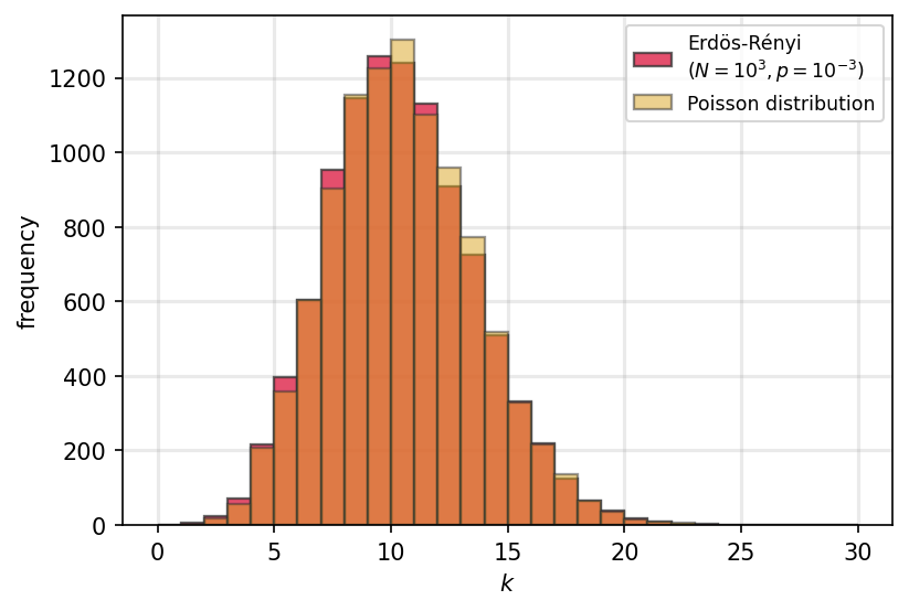
Erdős-Rényi Networks#
In the limit for large \(N\) the degree distribution \(P(k)\) can be approximated by the Poisson distribution:
Although, before that, it is defined by a Binomial distribution:
N = 10**4
p = 0.001
av_deg = (N-1)*p

num_bins = 20
bins = np.arange(0,31,1)

fig, ax = plt.subplots(1,1,figsize=(6,4),dpi=150)

g = nx.gnp_random_graph(N,p)
nd = np.array(list(dict(g.degree()).values()))

__ = ax.hist(nd, bins=bins, edgecolor='#333333', linewidth=1.1, color='crimson',
             alpha=0.75, label='Erdös-Rényi\n($N=10^{3}, p=10^{-3}$)')

k = np.random.poisson(av_deg, size=N)
__ = ax.hist(k, bins=bins, edgecolor='#333333', linewidth=1.1, color='goldenrod',
             alpha=0.5, label='Poisson distribution')

ax.legend(fontsize='small')
ax.grid(linewidth=1.5, color='#999999', alpha=0.2, linestyle='-')

ax.set_xlabel(r"$k$")
ax.set_ylabel("frequency")

plt.savefig('images/pngs/Pk_ER_vs_poisson.png', dpi=425, bbox_inches='tight')
plt.savefig('images/pdfs/Pk_ER_vs_poisson.pdf', bbox_inches='tight')
plt.show()

### Question: How do we generate poisson distributions without sampling + histograms?
###           What does this function do?
# from scipy.stats import poisson
Beyond Random Graphs#
Recall, from our last class:#
Source: Adamic, L. A., & Glance, N. (2005). The political blogosphere and the 2004 US election: Divided they blog. In Proceedings of the 3rd International Workshop on Link Discovery (pp. 36-43).
In the following we will learn how to load a directed graph, extract a vertex-induced subgraph, and compute the in- and out-degree of the vertices of the graph. We will use a directed graph that includes a collection of hyperlinks between weblogs on US politics, recorded in 2005 by Adamic and Glance.
The data are included in two tab-separated files:
polblogs_nodes.tsv: node id, node label, political orientation (0 = left or liberal, 1 = right or conservative).polblogs_edges.tsv: source node id, target node id.
Step-by-step way to make this network:#
One-by-one add nodes (blogs)
Connect nodes based on hyperlinks between blogs
digraph = nx.DiGraph()
with open('data/polblogs_nodes_class.tsv','r') as fp:
for line in fp:
node_id, node_label, node_political = line.strip().split('\t')
political_orientation = 'liberal' if node_political == '0' else 'conservative'
digraph.add_node(node_id, website=node_label, political_orientation=political_orientation)
with open('data/polblogs_edges_class.tsv','r') as fp:
for line in fp:
source_node_id, target_node_id = line.strip().split('\t')
digraph.add_edge(source_node_id, target_node_id)
degree = digraph.degree()
in_degree = digraph.in_degree()
out_degree = digraph.out_degree()
# I ususally make this a dictionary straight away
degree = dict(degree)
in_degree = dict(in_degree)
out_degree = dict(out_degree)
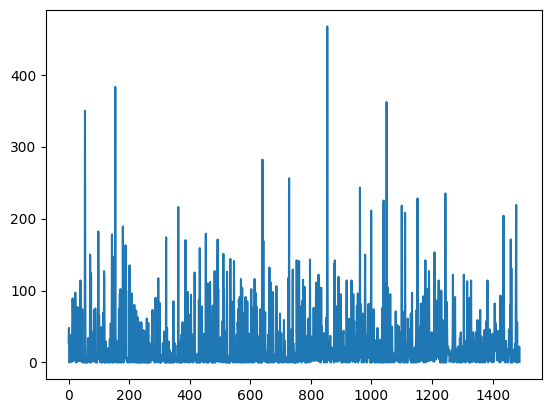
deg_vals = list(degree.values())
in_deg_vals = list(in_degree.values())
out_deg_vals = list(out_degree.values())
plt.plot(deg_vals)
[<matplotlib.lines.Line2D at 0x7f1adb134d10>]
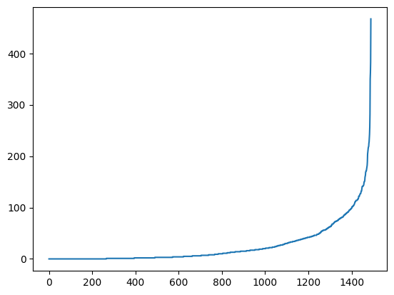
plt.plot(sorted(deg_vals))
[<matplotlib.lines.Line2D at 0x7f1adc267d50>]
from collections import Counter
min_deg = 0
max_deg = max(deg_vals)
deg_bins = {i:0 for i in range(min_deg, max_deg+1)}
for i,j in dict(Counter(deg_vals)).items():
    deg_bins[i] += j
plt.plot(list(deg_bins.keys()),list(deg_bins.values()))
[<matplotlib.lines.Line2D at 0x7f1adc299a10>]
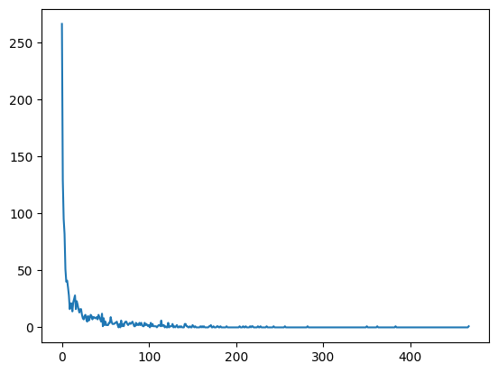
Question: Is this the most informative way to visualize this distribution?
Starting the class out with a challenge#
def degree_distribution(G, number_of_bins=15, log_binning=True, density=True, directed=False):
    """
    Given a degree sequence, return the y values (probability) and the
    x values (support) of a degree distribution that you're going to plot.

    Parameters
    ----------
    G (nx.Graph):
        the network whose degree distribution to calculate

    number_of_bins (int):
        length of output vectors

    log_binning (bool):
        if you are plotting on a log-log axis, then this is useful

    density (bool):
        whether to return counts or probability density (default: True)
        Note: probability densities integrate to 1 but do not sum to 1.

    directed (bool or str):
        if False, this assumes the network is undirected. Otherwise, the
        function requires an 'in' or 'out' as input, which will create the
        in- or out-degree distributions, respectively.

    Returns
    -------
    bins_out, probs (np.ndarray):
        probability density if density=True node counts if density=False; binned edges

    """

    # Step 0: Do we want the directed or undirected degree distribution?
    if directed:
        if directed=='in':
            pass

        elif directed=='out':
            pass

        else:
            out_error = "Help! if directed!=False, the input needs to be either 'in' or 'out'"
            print(out_error)
            # Question: Is this the correct way to raise an error message in Python?
            #           See "raise" function...
            return out_error
    else:
        pass


    # Step 1: We will first need to define the support of our distribution
    kmax = np.max(k)    # get the maximum degree
    kmin = 0            # let's assume kmin must be 0


    # Step 2: Then we'll need to construct bins
    if log_binning:
        pass
    else:
        pass


    # Step 3: Then we can compute the histogram using numpy


    # Step 4: Return not the "bins" but the midpoint between adjacent bin
    #         values. This is a better way to plot the distribution.


    pass

    return bins_out, probs
Plotting Degree Distributions#
The degree distribution \(P(k)\) of undirected graphs is defined as the probability that any randomly chosen vertex has degree \(k\).
In directed graphs, we need to consider two distributions: the in-degree \(P(k_{in})\) and out-degree \(P(k_{out})\) distributions, defined as the probability that a randomly chosen vertex has in-degree \(k_{in}\) and out-degree \(k_{out}\), respectively.
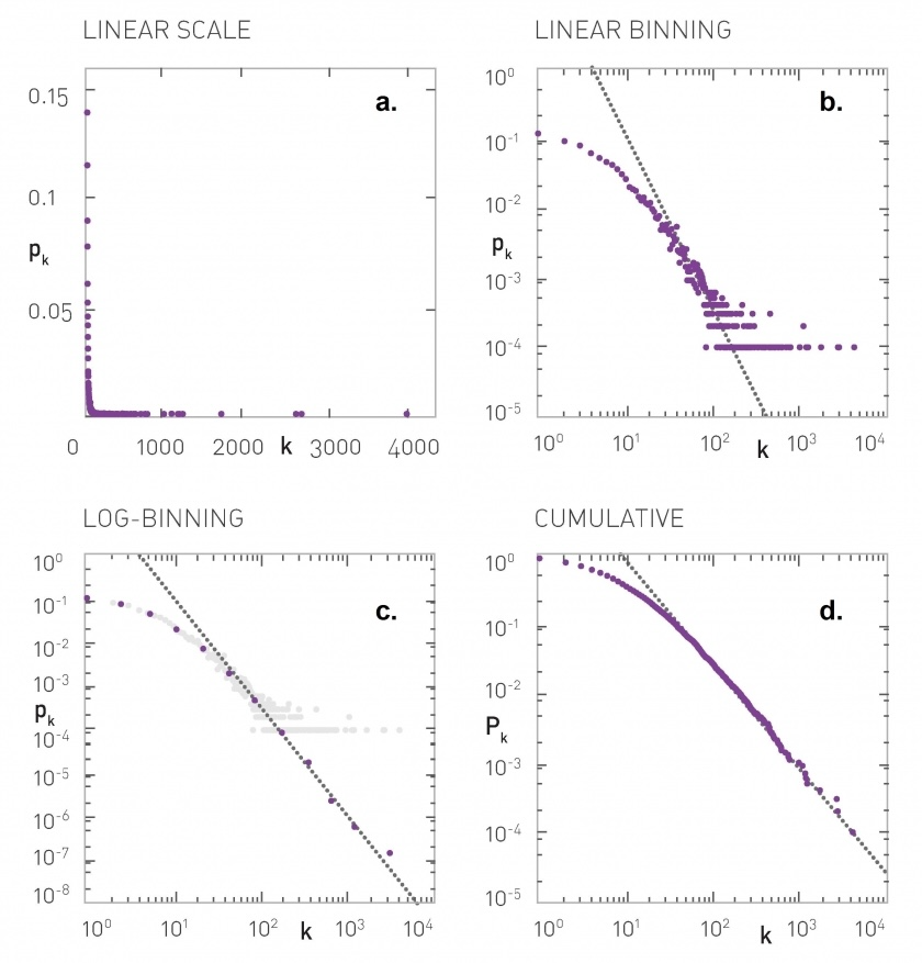
In many real world networks, degree distributions are skewed and highly variable (i.e. the support of the distribution spans several orders of magnitude). In many cases, this heavy tailed behavior can be approximated by a power-law decay \(P(k)\sim k^{-\alpha}\).
 Source: http://barabasi.com/networksciencebook/chapter/4#hubs
;) don’t look below
def degree_distribution(G, number_of_bins=15, log_binning=True, density=True, directed=False):
    """
    Given a degree sequence, return the y values (probability) and the
    x values (support) of a degree distribution that you're going to plot.

    Parameters
    ----------
    G (nx.Graph):
        the network whose degree distribution to calculate

    number_of_bins (int):
        length of output vectors

    log_binning (bool):
        if you are plotting on a log-log axis, then this is useful

    density (bool):
        whether to return counts or probability density (default: True)
        Note: probability densities integrate to 1 but do not sum to 1.

    directed (bool or str):
        if False, this assumes the network is undirected. Otherwise, the
        function requires an 'in' or 'out' as input, which will create the
        in- or out-degree distributions, respectively.

    Returns
    -------
    bins_out, probs (np.ndarray):
        probability density if density=True node counts if density=False; binned edges

    """

    # Step 0: Do we want the directed or undirected degree distribution?
    if directed:
        if directed=='in':
            k = list(dict(G.in_degree()).values()) # get the in degree of each node
        elif directed=='out':
            k = list(dict(G.out_degree()).values()) # get the out degree of each node
        else:
            out_error = "Help! if directed!=False, the input needs to be either 'in' or 'out'"
            print(out_error)
            # Question: Is this the correct way to raise an error message in Python?
            #           See "raise" function...
            return out_error
    else:
        k = list(dict(G.degree()).values()) # get the degree of each node


    # Step 1: We will first need to define the support of our distribution
    kmax = np.max(k)    # get the maximum degree
    kmin = 0            # let's assume kmin must be 0


    # Step 2: Then we'll need to construct bins
    if log_binning:
        # array of bin edges including rightmost and leftmost
        bins = np.logspace(0, np.log10(kmax+1), number_of_bins+1)
    else:
        bins = np.linspace(0, kmax+1, num=number_of_bins+1)


    # Step 3: Then we can compute the histogram using numpy
    probs, _ = np.histogram(k, bins, density=density)


    # Step 4: Return not the "bins" but the midpoint between adjacent bin
    #         values. This is a better way to plot the distribution.
    bins_out = bins[1:] - np.diff(bins)/2.0

    return bins_out, probs
G0 = nx.to_undirected(digraph)
x, y = degree_distribution(G0)
print(len(x),len(y))

plt.loglog(x, y,marker='o',lw=0);
15 15

x_in, y_in = degree_distribution(digraph, number_of_bins=80, log_binning=True, directed='in')
x_out,y_out = degree_distribution(digraph, number_of_bins=80, log_binning=True, directed='out')
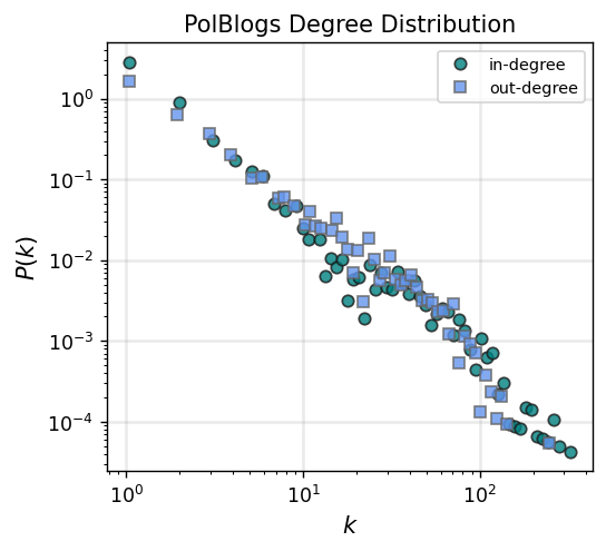
fig, ax = plt.subplots(1,1,figsize=(4.5,4),dpi=125)
ax.loglog(x_in, y_in,'o', color='teal', label='in-degree', alpha=0.8, mec='.1')
ax.loglog(x_out, y_out,'s', color='cornflowerblue', label='out-degree', alpha=0.8, mec='.4')
ax.set_xlabel(r"$k$",fontsize='large')
ax.set_ylabel(r"$P(k)$",fontsize='large')
ax.legend(fontsize='small')
ax.grid(linewidth=1.5, color='#999999', alpha=0.2, linestyle='-')
ax.set_title('PolBlogs Degree Distribution')
plt.savefig('images/pngs/PolBlogs_inout_degreedist.png', dpi=425, bbox_inches='tight')
plt.savefig('images/pdfs/PolBlogs_inout_degreedist.pdf', bbox_inches='tight')
plt.show()
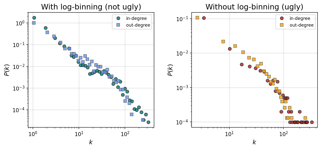
# Note: your plots will look stupid if you don't do log binning...
nbins = 50
fig, ax = plt.subplots(1,2,figsize=(10,4),dpi=150)
plt.subplots_adjust(wspace=0.3)

x_in, y_in  = degree_distribution(digraph, number_of_bins=nbins, log_binning=True, directed='in')
x_out,y_out = degree_distribution(digraph, number_of_bins=nbins, log_binning=True, directed='out')
ax[0].loglog(x_in, y_in, 'o', color='teal', label='in-degree', alpha=0.8, mec='.1')
ax[0].loglog(x_out, y_out, 's', color='cornflowerblue', label='out-degree', alpha=0.8, mec='.4')
ax[0].set_xlabel(r"$k$", fontsize='large')
ax[0].set_ylabel(r"$P(k)$", fontsize='large')
ax[0].legend(fontsize='small')
ax[0].grid(linewidth=1.5, color='#999999', alpha=0.2, linestyle='-')
ax[0].set_title('With log-binning (not ugly)', fontsize='x-large')

x_in, y_in  = degree_distribution(digraph, number_of_bins=nbins, log_binning=False, directed='in')
x_out,y_out = degree_distribution(digraph, number_of_bins=nbins, log_binning=False, directed='out')
ax[1].loglog(x_in, y_in, 'o', color='firebrick', label='in-degree', alpha=0.8, mec='.1')
ax[1].loglog(x_out, y_out, 's', color='orange', label='out-degree', alpha=0.8, mec='.4')
ax[1].set_xlabel(r"$k$", fontsize='large')
ax[1].set_ylabel(r"$P(k)$", fontsize='large')
ax[1].legend(fontsize='small')
ax[1].grid(linewidth=1.5, color='#999999', alpha=0.2, linestyle='-')
ax[1].set_title('Without log-binning (ugly)', fontsize='x-large')

plt.savefig('images/pngs/PolBlogs_inout_degreedist_binningcompare.png', dpi=425, bbox_inches='tight')
plt.savefig('images/pdfs/PolBlogs_inout_degreedist_binningcompare.pdf', bbox_inches='tight')
plt.show()
Note from Advanced Topics 4b in Network Science by Lászlo Barabási#
https://networksciencebook.com/chapter/4#advanced-b
Using the network generator functions from last class…#
Your Turn!
Generate 3 random graphs with roughly the same number of nodes and edges that the
polblogsdataset hasPlot the degree distribution in the same plot as the true degree distribution
Write a few sentences that show what you’ve found
N = G0.number_of_nodes()
E = G0.number_of_edges()
print(N,E)
1490 16718
G1 = nx.gnm_random_graph(N,E) # same number of nodes and edges
G2 = nx.powerlaw_cluster_graph(N, 11, p=0.01) # same number of nodes, similar number of edges
G3 = nx.duplication_divergence_graph(N, 0.6698) # had to work at it, but approx same number of nodes + edges
# np.mean([nx.duplication_divergence_graph(N, 0.6698).number_of_edges() for i in range(100)])
fig, ax = plt.subplots(1,1,figsize=(6,4),dpi=100)

x0,y0 = degree_distribution(G0, number_of_bins=12)
x1,y1 = degree_distribution(G1, number_of_bins=12)
x2,y2 = degree_distribution(G2, number_of_bins=12)
x3,y3 = degree_distribution(G3, number_of_bins=12)

ax.loglog(x0,y0,marker='o',lw=0.5,ls=':',label='polblogs')
ax.loglog(x1,y1,marker='s',lw=0.5,ls=':',label=r'$G_{n,m}$')
ax.loglog(x2,y2,marker='^',lw=0.5,ls=':',label='powerlaw cluster')
ax.loglog(x3,y3,marker='X',lw=0.5,ls=':',label='duplication divergence')

ax.legend(fontsize='small')
ax.set_xlabel(r'$k$',fontsize='x-large')
ax.set_ylabel(r'$P(k)$',fontsize='x-large')

plt.show()

Paths and Components#
Let us defines a path \(P_{i_0,i_n}\) in a graph \(G = (V,E)\) as an ordered collection of vertices \(\{i_0, i_1, \dots, i_n \}\) and \(n\) edges \(\{(i_0,i_1), (i_1,i_2), \dots, (i_{n-1},i_n) \}\) such that \(i_a \in V\) and \((i_{a-1},i_a) \in E, \forall a\). The path \(P_{i_0,i_n}\) connects nodes \(i_0\) and \(i_n\) and its length is \(n\).
Note: The number of paths of length \(n\) between two nodes \(i\) and \(j\) is equivalent to the element \(i,j\) of the \(n\)th power of the adjacency matrix \(A\).
A shortest-path (or geodesic path) is the shortest path connecting two vertices.
The eccentricity \(\epsilon\) of a vertex \(i\) is the longest shortest-path between vertex \(i\) and any other vertex \(j\).
The radius \(r\) of a graph \(G=(V,E)\) is the minimum eccentricity of any node in \(V\).
The diameter \(d\) of a graph \(G=(V,E)\) is the maximum eccentricity of any node in \(V\).
A cycle (or loop) is a closed path (i.e. \(i_0 = i_n\)) in which all vertices and all edges are distinct. If a graph \(G=(V,E)\) does not contain any cycle, than such graph is said to be acyclic. Instead, if it contains at least one cycle, the graph is said to be cyclic.
We’ll be diving into paths more thoroughly in later lessons, but to kick things off today, let’s define these terms above…
Starting with shortest path.
G = nx.karate_club_graph()
Question: What is our “shortest path” function meant to do?
Goal: I want to know the shortest path from node i to node j.
Goal: I want to know the shortest paths from all nodes i to all other nodes j.
node_i = 0
# For a given node i, let's initialize all other nodes to be -1 (infinite) hops away
distances = {i: -1 for i in G.nodes()}

# And distance of 0 from node_i to itself
distances[node_i] = 0

# I'll need to make a queue of nodes to search... How to do this?
pass
Breadth-first search (BFS)#
# Queue of nodes to visit next, starting with our source node_i
queue = [node_i]

# We want to:
### 1. Start with one element in our queue
### 2. Find its neighbors and add them to our queue
### 3. Select one of the neighbors from the queue
### 4. Add its neighbors to our queue
### 5. And so on, until the queue has been depleted

# This is a great time for a `while` loop!

# while there is still a queue of any positive length (instead of len(queue)>0)...
while queue:
    # select oldest item in the list (as opposed to last item)
    current_node = queue.pop(0)

    # find all the
    for next_node in G.neighbors(current_node):
        if distances[next_node] < 0:
            # set next_node's distance to be +1 whatever the distance to the current node is
            ### e.g. if current_node distance is 0, its neighbors will be 0+1 distance away
            ### ... and so on
            distances[next_node] = distances[current_node] + 1

            # and since we havent seen next_node before (distance still < 0)
            # we will need to append it to our queue
            queue.append(next_node)
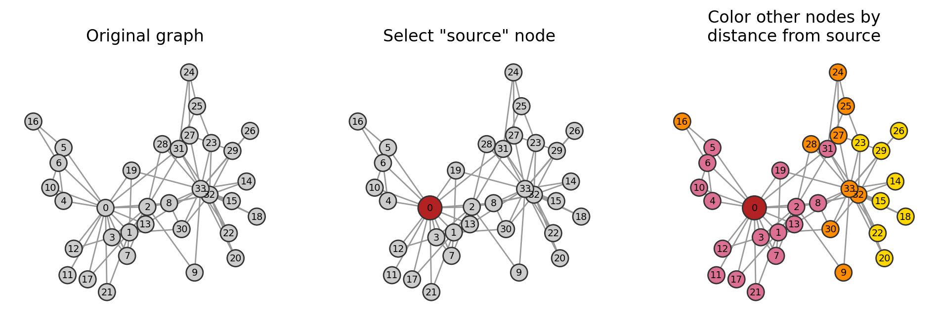
pos = nx.spring_layout(G)
fig, ax = plt.subplots(1,3,figsize=(12,3.5),dpi=200)

dist_col_map = {0:'firebrick',
                1:'palevioletred',
                2:'darkorange',
                3:'gold'}

node_cols0 = ['.8' for i in G.nodes()]
nx.draw(G, pos, node_size=150, node_color=node_cols0, edgecolors='.2',
        with_labels=True, font_size='x-small', edge_color='.6', ax=ax[0])

node_cols1 = ['firebrick' if i==node_i else '.8' for i in G.nodes()]
nx.draw(G, pos, node_size=[300 if i==node_i else 150 for i in G.nodes()],
        node_color=node_cols1, edgecolors='.2',
        with_labels=True, font_size='x-small', edge_color='.6', ax=ax[1])

node_cols2 = [dist_col_map[i] for i in distances.values()]
nx.draw(G, pos, node_size=[300 if i==node_i else 150 for i in G.nodes()],
        node_color=node_cols2, edgecolors='.2',
        with_labels=True, font_size='x-small', edge_color='.6', ax=ax[2])

ax[0].set_title('Original graph')
ax[1].set_title('Select "source" node')
ax[2].set_title('Color other nodes by\ndistance from source')


plt.savefig('images/pngs/networkx_example_BFS.png', dpi=425, bbox_inches='tight')
plt.savefig('images/pdfs/networkx_example_BFS.pdf', bbox_inches='tight')

plt.show()
Putting it all together#
Your turn!
Finish the function all_shortest_from below. We’ll need it for an exercise shortly.
def all_shortest_from(G, node_i):
    """
    For a given node_i in the network, construct a dictionary containing
    the length of the shortest path between that node and all others in
    the network. Values of -1 correspond to nodes where no paths connect
    to node_i.

    Parameters
    ----------
    G (nx.Graph)
        the graph in question

    node_i (int or str)
        the label of the "source" node

    Returns
    -------
    distances (dict)
        dictionary where the key corresponds to other nodes in the network
        and the values indicate the shortest path length between that node
        and the original node_i source.

    """

    pass

    return distances
def all_shortest_from(G, node_i):
    """
    For a given node_i in the network, construct a dictionary containing
    the length of the shortest path between that node and all others in
    the network. Values of -1 correspond to nodes where no paths connect
    to node_i.

    Parameters
    ----------
    G (nx.Graph)
        the graph in question

    node_i (int or str)
        the label of the "source" node

    Returns
    -------
    distances (dict)
        dictionary where the key corresponds to other nodes in the network
        and the values indicate the shortest path length between that node
        and the original node_i source.

    """

    distances = {i: -1 for i in G.nodes()}

    # And distance of 0 from node_i to itself
    distances[node_i] = 0

    # Queue of nodes to visit next, starting with our source node_i
    queue = [node_i]

    # We want to:
    ### 1. Start with one element in our queue
    ### 2. Find its neighbors and add them to our queue
    ### 3. Select one of the neighbors from the queue
    ### 4. Add its neighbors to our queue
    ### 5. And so on, until the queue has been depleted

    # This is a great time for a `while` loop!

    # while there is still a queue of any positive length (instead of len(queue)>0)...
    while queue:
        # select oldest item in the list (as opposed to last item)
        current_node = queue.pop(0)

        # find all the
        for next_node in G.neighbors(current_node):
            if distances[next_node] < 0:
                # set next_node's distance to be +1 whatever the distance to the current node is
                ### e.g. if current_node distance is 0, its neighbors will be 0+1 distance away
                ### ... and so on
                distances[next_node] = distances[current_node] + 1

                # and since we havent seen next_node before (distance still < 0)
                # we will need to append it to our queue
                queue.append(next_node)

    return distances
From above:#
A shortest-path (or geodesic path) is the shortest path connecting two vertices.
The eccentricity \(\epsilon\) of a vertex \(i\) is the longest shortest-path between vertex \(i\) and any other vertex \(j\).
The radius \(r\) of a graph \(G=(V,E)\) is the minimum eccentricity of any node in \(V\).
The diameter \(d\) of a graph \(G=(V,E)\) is the maximum eccentricity of any node in \(V\).
A cycle (or loop) is a closed path (i.e. \(i_0 = i_n\)) in which all vertices and all edges are distinct. If a graph \(G=(V,E)\) does not contain any cycle, than such graph is said to be acyclic. Instead, if it contains at least one cycle, the graph is said to be cyclic.
Your turn!
Use your function
all_shortest_pathsabove to compute the shortest path lengths for every node inG.Use this to calculate the following:
A) The eccentrity of all nodes in
GB) The radius of
GC) The diameter of
G
Cross-reference your answer with the output from
networkx.
pass
print("Radius:",nx.radius(G))
print("Diameter:",nx.diameter(G))
print(nx.eccentricity(G))
Radius: 3
Diameter: 5
{0: 3, 1: 3, 2: 3, 3: 3, 4: 4, 5: 4, 6: 4, 7: 4, 8: 3, 9: 4, 10: 4, 11: 4, 12: 4, 13: 3, 14: 5, 15: 5, 16: 5, 17: 4, 18: 5, 19: 3, 20: 5, 21: 4, 22: 5, 23: 5, 24: 4, 25: 4, 26: 5, 27: 4, 28: 4, 29: 5, 30: 4, 31: 3, 32: 4, 33: 4}
Segue: A special kind of “path”#
Remember from above: The number of paths of length \(l\) between two nodes \(i\) and \(j\) in a graph can be found in the \(ij^{th}\) element of the \(l^{th}\) power of the adjacency matrix \(A\).
A = nx.to_numpy_array(G, weight=None)
A
array([[0., 1., 1., ..., 1., 0., 0.],
       [1., 0., 1., ..., 0., 0., 0.],
       [1., 1., 0., ..., 0., 1., 0.],
       ...,
       [1., 0., 0., ..., 0., 1., 1.],
       [0., 0., 1., ..., 1., 0., 1.],
       [0., 0., 0., ..., 1., 1., 0.]])
# recall that matrix multiplication in numpy is done as follows:
A @ A
array([[16.,  7.,  5., ...,  0.,  3.,  4.],
       [ 7.,  9.,  4., ...,  1.,  2.,  3.],
       [ 5.,  4., 10., ...,  3.,  1.,  6.],
       ...,
       [ 0.,  1.,  3., ...,  6.,  1.,  2.],
       [ 3.,  2.,  1., ...,  1., 12., 10.],
       [ 4.,  3.,  6., ...,  2., 10., 17.]])
Take a moment to interpret what this is showing.
What do the diagonal elements correspond to?
What do the off-diagonal elements correspond to?
Is this matrix symmetric?
What if we take the third power, \(A^3\), of the adjacency matrix?
A @ A @ A
array([[36., 37., 42., ..., 27., 12., 14.],
       [37., 24., 34., ..., 13., 11., 13.],
       [42., 34., 22., ..., 13., 32., 22.],
       ...,
       [27., 13., 13., ...,  6., 31., 36.],
       [12., 11., 32., ..., 31., 26., 40.],
       [14., 13., 22., ..., 36., 40., 30.]])
How does this operation relate to the networkx function nx.triangles?
pass
Clustering#
Node degree tells us how many neighbors each vertex has. However, we might also want to know how one node’s neighbors are related to each other. We can intuit this by imagining paths of length three in our graph. The concept of clustering (or transitivity in the context of sociology) refers exaclty to this: the tendency for nodes to form cliques around a given vertex.
Local Clustering#
Given an undirected graph \(G=(V,E)\), let us define the local clustering coefficient as the probability that any two neighbors \(j\) and \(k\) of node \(i\) are connected:
where \(k_i\) is the degree of node \(i\) and \(e_i\) the number of edges that exists between the neighbors of node \(i\). In other words, the clustering coefficient of a node represents the ratio between the number of triangles in the subgraph \(G'\) induced by node \(i\) and its neighbors over the number of all possible triangles that would be present if \(G'\) was a complete graph.
The average clustering coefficient of a network, then, is simply: \(\langle C \rangle = \frac{1}{N}\sum_i C(i)\).
In directed graphs, the definition of clustering can be further refined since 8 different types of triangles can be present in our graph; see Fagiolo (2007).
G = nx.karate_club_graph()
# Step 1: Select a random node, i
i = 0

# Step 2: Get all the neighbors of node i
G.neighbors(i)

# Step 3: How do we get all the ***possible*** triangles?
<dict_keyiterator at 0x7f1adaf27b50>
Interlude: itertools — Functions creating iterators for efficient looping#
This module implements a number of iterator building blocks inspired by constructs from APL, Haskell, and SML. Each has been recast in a form suitable for Python.
The module standardizes a core set of fast, memory efficient tools that are useful by themselves or in combination. Together, they form an “iterator algebra” making it possible to construct specialized tools succinctly and efficiently in pure Python.
Source: https://docs.python.org/3/library/itertools.html
from itertools import combinations # Return successive r-length combinations of elements in the iterable.
list1 = [1,2,3,4,5]
r = 1

list(combinations(list1, r))
[(1,), (2,), (3,), (4,), (5,)]
r = 2
list(combinations(list1, r))
[(1, 2),
 (1, 3),
 (1, 4),
 (1, 5),
 (2, 3),
 (2, 4),
 (2, 5),
 (3, 4),
 (3, 5),
 (4, 5)]
node_i = 0
neighbors_i = list(G.neighbors(node_i))
print("node %i is connected to nodes:"%node_i,neighbors_i)
node 0 is connected to nodes: [1, 2, 3, 4, 5, 6, 7, 8, 10, 11, 12, 13, 17, 19, 21, 31]
possible_triangle_edges_i = list(combinations(neighbors_i,2))
print("The potential neighbor-neighbor edges among node %i's neighbors is:"%node_i,
      possible_triangle_edges_i, '\n\n(length = %i)'%len(possible_triangle_edges_i))
The potential neighbor-neighbor edges among node 0's neighbors is: [(1, 2), (1, 3), (1, 4), (1, 5), (1, 6), (1, 7), (1, 8), (1, 10), (1, 11), (1, 12), (1, 13), (1, 17), (1, 19), (1, 21), (1, 31), (2, 3), (2, 4), (2, 5), (2, 6), (2, 7), (2, 8), (2, 10), (2, 11), (2, 12), (2, 13), (2, 17), (2, 19), (2, 21), (2, 31), (3, 4), (3, 5), (3, 6), (3, 7), (3, 8), (3, 10), (3, 11), (3, 12), (3, 13), (3, 17), (3, 19), (3, 21), (3, 31), (4, 5), (4, 6), (4, 7), (4, 8), (4, 10), (4, 11), (4, 12), (4, 13), (4, 17), (4, 19), (4, 21), (4, 31), (5, 6), (5, 7), (5, 8), (5, 10), (5, 11), (5, 12), (5, 13), (5, 17), (5, 19), (5, 21), (5, 31), (6, 7), (6, 8), (6, 10), (6, 11), (6, 12), (6, 13), (6, 17), (6, 19), (6, 21), (6, 31), (7, 8), (7, 10), (7, 11), (7, 12), (7, 13), (7, 17), (7, 19), (7, 21), (7, 31), (8, 10), (8, 11), (8, 12), (8, 13), (8, 17), (8, 19), (8, 21), (8, 31), (10, 11), (10, 12), (10, 13), (10, 17), (10, 19), (10, 21), (10, 31), (11, 12), (11, 13), (11, 17), (11, 19), (11, 21), (11, 31), (12, 13), (12, 17), (12, 19), (12, 21), (12, 31), (13, 17), (13, 19), (13, 21), (13, 31), (17, 19), (17, 21), (17, 31), (19, 21), (19, 31), (21, 31)]

(length = 120)
Recall above: How many possible edges should we expect based on the equation above?
node_i = 0
k_i = G.degree(node_i)
print(k_i)
16
# according to the equation above, we know the denominator should be k_i(k_i-1)/2
possible_triangles_i = k_i * (k_i-1)/2
possible_triangles_i

# what is the numerator? **the number of edges between nodes that are neighbors of node_i**
120.0
actual_triangles_i = sum([1 for neigh_i,neigh_j in possible_triangle_edges_i
                          if neigh_j in G.neighbors(neigh_i)])
clustering_i = actual_triangles_i/possible_triangles_i
clustering_i
0.15
nx.clustering(G)[0]
0.15
clustering_dict = {}
for node_i in G.nodes():
    k_i = G.degree(node_i)
    neighbors_i = list(G.neighbors(node_i))

    possible_triangle_edges_i = list(combinations(neighbors_i,2))
    possible_triangles_i = k_i * (k_i-1) / 2

    actual_triangles_i = sum([1 for neigh_i,neigh_j in possible_triangle_edges_i
                              if neigh_j in G.neighbors(neigh_i)])

    if possible_triangles_i > 0:
        clustering_i = actual_triangles_i/possible_triangles_i
    else:
        clustering_i = 0.0

    clustering_dict[node_i] = clustering_i
clustering_dict
{0: 0.15,
 1: 0.3333333333333333,
 2: 0.24444444444444444,
 3: 0.6666666666666666,
 4: 0.6666666666666666,
 5: 0.5,
 6: 0.5,
 7: 1.0,
 8: 0.5,
 9: 0.0,
 10: 0.6666666666666666,
 11: 0.0,
 12: 1.0,
 13: 0.6,
 14: 1.0,
 15: 1.0,
 16: 1.0,
 17: 1.0,
 18: 1.0,
 19: 0.3333333333333333,
 20: 1.0,
 21: 1.0,
 22: 1.0,
 23: 0.4,
 24: 0.3333333333333333,
 25: 0.3333333333333333,
 26: 1.0,
 27: 0.16666666666666666,
 28: 0.3333333333333333,
 29: 0.6666666666666666,
 30: 0.5,
 31: 0.2,
 32: 0.19696969696969696,
 33: 0.11029411764705882}
nx.clustering(G)
{0: 0.15,
 1: 0.3333333333333333,
 2: 0.24444444444444444,
 3: 0.6666666666666666,
 4: 0.6666666666666666,
 5: 0.5,
 6: 0.5,
 7: 1.0,
 8: 0.5,
 9: 0,
 10: 0.6666666666666666,
 11: 0,
 12: 1.0,
 13: 0.6,
 14: 1.0,
 15: 1.0,
 16: 1.0,
 17: 1.0,
 18: 1.0,
 19: 0.3333333333333333,
 20: 1.0,
 21: 1.0,
 22: 1.0,
 23: 0.4,
 24: 0.3333333333333333,
 25: 0.3333333333333333,
 26: 1.0,
 27: 0.16666666666666666,
 28: 0.3333333333333333,
 29: 0.6666666666666666,
 30: 0.5,
 31: 0.2,
 32: 0.19696969696969696,
 33: 0.11029411764705882}
np.mean(list(clustering_dict.values()))
0.5706384782076823
nx.average_clustering(G)
0.5706384782076823
Global Clustering#
The global clustering coefficient measures the total number of closed triangles in a network relative to the number of existing connected triplets (i.e. the number of not closed triangles):
where a connected triplet is an ordered set of three vertices.
networkx has a function for this! It’s (depending on your scholarly background) counter-intuitively named nx.transitivity.
nx.transitivity(G)
0.2556818181818182
How can we compute this from scratch using what we know about graph properties so far?
A3 = A@A@A
A3
array([[36., 37., 42., ..., 27., 12., 14.],
       [37., 24., 34., ..., 13., 11., 13.],
       [42., 34., 22., ..., 13., 32., 22.],
       ...,
       [27., 13., 13., ...,  6., 31., 36.],
       [12., 11., 32., ..., 31., 26., 40.],
       [14., 13., 22., ..., 36., 40., 30.]])
num_triangles = int(np.trace(A3)/6)
print(num_triangles)
45
degrees = dict(G.degree())
connected_triplets = sum(deg * (deg - 1) // 2 for deg in degrees.values())
print(connected_triplets)
528
global_clustering = 3 * num_triangles / connected_triplets
print(global_clustering)
0.2556818181818182
Your turn!#
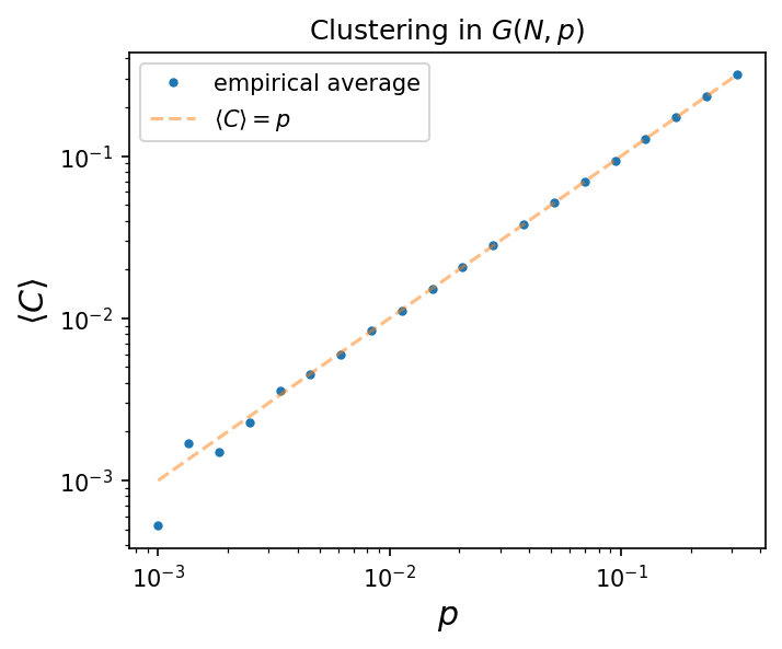
Graphs sampled from \(G(N,p)\) do not have clustering. Why is that?
The average clustering coefficient in \(G(N,p)\) is \( \langle C \rangle = p = \frac{\langle k \rangle}{N}. \) Show this numerically.
(Warning: The code block below takes a few minutes to run…)
N = 500
ps = np.logspace(-3,-0.5,20)
niter = 100
clustering = []

for p in ps:
    tmp = []
    for _ in range(niter):
        G_i = nx.erdos_renyi_graph(N,p)
        tmp.append(nx.transitivity(G_i))

    clustering.append(np.mean(tmp))
---------------------------------------------------------------------------
KeyboardInterrupt                         Traceback (most recent call last)
Cell In[53], line 9
      7 tmp = []
      8 for _ in range(niter):
----> 9     G_i = nx.erdos_renyi_graph(N,p)
     10     tmp.append(nx.transitivity(G_i))
     12 clustering.append(np.mean(tmp))

File <class 'networkx.utils.decorators.argmap'> compilation 5:4, in argmap_gnp_random_graph_1(n, p, seed, directed, create_using, backend, **backend_kwargs)
      2 import collections
      3 import gzip
----> 4 import inspect
      5 import itertools
      6 import re

File /opt/hostedtoolcache/Python/3.11.13/x64/lib/python3.11/site-packages/networkx/utils/backends.py:535, in _dispatchable._call_if_no_backends_installed(self, backend, *args, **kwargs)
    529 if "networkx" not in self.backends:
    530     raise NotImplementedError(
    531         f"'{self.name}' is not implemented by 'networkx' backend. "
    532         "This function is included in NetworkX as an API to dispatch to "
    533         "other backends."
    534     )
--> 535 return self.orig_func(*args, **kwargs)

File /opt/hostedtoolcache/Python/3.11.13/x64/lib/python3.11/site-packages/networkx/generators/random_graphs.py:180, in gnp_random_graph(n, p, seed, directed, create_using)
    178 edgetool = itertools.permutations if directed else itertools.combinations
    179 for e in edgetool(range(n), 2):
--> 180     if seed.random() < p:
    181         G.add_edge(*e)
    182 return G

KeyboardInterrupt:
fig, ax = plt.subplots(1,1,figsize=(5,4),dpi=150)

ax.loglog(ps, clustering, marker='.', lw=0, label='empirical average')
ax.loglog(ps, ps, label=r'$\langle C \rangle = p$', alpha=0.5, ls='--')

ax.legend()
ax.set_xlabel(r'$p$', fontsize='x-large')
ax.set_ylabel(r'$\langle C \rangle$', fontsize='x-large')

ax.set_title(r'Clustering in $G(N,p)$')

plt.show()
Want more? In your own time…#
The weighted clustering of node \(i\) in an undirected weighted graph \(G\) can be defined as:
where \(s_i\) is the stength of node \(i\), \(k_i\) is the degree of node \(i\), and \(w_{ij}\) is the weight associated to the edge connecting nodes \(i\) and \(j\).
Write a function that computes the weighted clusterings \(C^w(i)\) for all nodes in an undirected weighted graph.
pass
Use a depth-first search (DFS) to find connected components in a graph.
Below is an example of the order that nodes are searched in DFS.

And a helpful gif:

pass
Next time…#
Degree, path lengths, triangles: these are all different ways to understand an individual node’s role/status/importance in networks. Next time, we’ll start to ask about distributions of network properties & explore even more centralities! class_04_distributions.ipynb
References and further resources:#
Class Webpages
Jupyter Book: https://asmithh.github.io/network-science-data-book/intro.html
Syllabus and course details: https://brennanklein.com/phys7332-fall24
Fagiolo, G. (2007). Clustering in complex directed networks. Physical Review E, 76(2), 026107.
Network Science textbook (https://networksciencebook.com/).
Watts, D.J. & Strogatz, S.H. (1998). Collective dynamics of ‘small-world’ networks. Nature, 393: 409–10.