Class 8: Data Science 1 — Pandas, SQL, Regressions#
Come in. Sit down. Open Teams.
Make sure your notebook from last class is saved.
Open up the Jupyter Lab server.
Open up the Jupyter Lab terminal.
Activate Conda:
module load anaconda3/2022.05Activate the shared virtual environment:
source activate /courses/PHYS7332.202510/shared/phys7332-env/Run
python3 git_fixer2.pyGithub:
git status (figure out what files have changed)
git add … (add the file that you changed, aka the
_MODIFIEDone(s))git commit -m “your changes”
git push origin main
Goals of today’s class#
Get comfortable using
pandasfor tabular dataLearn how to use basic SQL commands
Understand how regressions work at a very high level.
Pandas#
Adapted from 10 minutes to pandas
pandas is a Python library for manipulating & analyzing data.
We usually import pandas like this:
import pandas as pd
pandas has two basic units that we care about: a Series and a DataFrame. Series are roughly akin to lists – they’re one-dimensional and can hold data of any type. DataFrames are two-dimensional (they have rows and columns) and are indexed by one or more columns. This means that a row can be identified by the labels in the index column. Each column of a DataFrame is also a Series.
We’ll focus on DataFrames for now. We can populate a DataFrame in a few different ways. First, let’s instantiate a DataFrame with our own data.
Making a DataFrame:#
df = pd.DataFrame({
    "Name": ["Orca", "Blue Whale", "Beluga Whale", "Narwhal"],
    "Weight": [22000, 441000, 2530, 3500],
    "Cute":[True, True, True, True],
    "Habitat": ["Everywhere", "Everywhere", "Arctic", "Arctic"],
})
Let’s look at the types the columns of df have:
df.dtypes
Name       object
Weight      int64
Cute         bool
Habitat    object
dtype: object
Wow! These are a lot of different types!
We can also access the column names like this:
df.columns
Index(['Name', 'Weight', 'Cute', 'Habitat'], dtype='object')
or see the first 3 entries like this:
df.head(3)
| Name | Weight | Cute | Habitat | |
|---|---|---|---|---|
| 0 | Orca | 22000 | True | Everywhere |
| 1 | Blue Whale | 441000 | True | Everywhere |
| 2 | Beluga Whale | 2530 | True | Arctic |
Common Pandas operations#
Sorting#
Now we’ll practice some common operations in pandas. One thing we might want to do is sort a dataframe by a particular column:
df.sort_values(by="Weight", ascending=False)
| Name | Weight | Cute | Habitat | |
|---|---|---|---|---|
| 1 | Blue Whale | 441000 | True | Everywhere |
| 0 | Orca | 22000 | True | Everywhere |
| 3 | Narwhal | 3500 | True | Arctic |
| 2 | Beluga Whale | 2530 | True | Arctic |
What happens if we change the ascending parameter to True?
Can you sort the dataframe alphabetically by species name?
# Your turn!!!
Filtering#
Another common thing we can do in Pandas is filtering. This means we only select the rows that match a specific condition. Let’s filter for all the cetaceans whose weight is over 5000 pounds:
df[df.Weight > 5000]
| Name | Weight | Cute | Habitat | |
|---|---|---|---|---|
| 0 | Orca | 22000 | True | Everywhere |
| 1 | Blue Whale | 441000 | True | Everywhere |
Here, we’re referring to the Weight column as an attribute of our dataframe df. However, we can also refer to the column like we would a key in a dictionary, with the same result:
df[df['Weight'] > 5000]
| Name | Weight | Cute | Habitat | |
|---|---|---|---|---|
| 0 | Orca | 22000 | True | Everywhere |
| 1 | Blue Whale | 441000 | True | Everywhere |
Can you filter the dataframe to get all the cetaceans that live in the Arctic?
# Your turn!!
Adding a column#
We can also add a column to the dataframe as long as it’s the same length as the existing dataframe:
df["Food"] = ["Everything", "Krill", "Squid, Clams, Octopus, Cod, Herring", "Fish"]
And we can create a column from an existing column using the apply function:
def convert_from_lbs_to_kg(wt):
    return wt * 0.45
df["Weight_kg"] = df["Weight"].apply(convert_from_lbs_to_kg)
When we apply a function, we can use an actual function, as we did above, or we can use an anonymous function, or a “lambda function”.
df["Weight_tons"] = df["Weight"].apply(lambda b: b / 2000)
Grouping#
We also might want to group our dataframe into chunks that have something in common.
groups = df.groupby('Habitat')
for habitat, df_gr in groups:
    print(habitat)
    print(df_gr.head())
Arctic
           Name  Weight  Cute Habitat                                 Food  \
2  Beluga Whale    2530  True  Arctic  Squid, Clams, Octopus, Cod, Herring
3       Narwhal    3500  True  Arctic                                 Fish

   Weight_kg  Weight_tons
2     1138.5        1.265
3     1575.0        1.750
Everywhere
         Name  Weight  Cute     Habitat        Food  Weight_kg  Weight_tons
0        Orca   22000  True  Everywhere  Everything     9900.0         11.0
1  Blue Whale  441000  True  Everywhere       Krill   198450.0        220.5
Here, we’re grouping our dataframe by the Habitat column. groups is an iterable (we can iterate over the items in it, in the order given to us) that has two variables. One of them is the unique value of the column we grouped by (Everywhere and Arctic) and the other one is the chunk of the dataframe that had that unique value in that column.
Can you group the cetaceans that weigh more than 5000 pounds apart from the ones that weigh less than 5000 pounds? (Hint: You might have to create a new column!)
# Your Turn!!!
Practicing with Pandas#
We can also load a pandas dataframe from a .csv (comma separated values) file. We’re going to load up WhaleFromSpaceDB_Whales.csv, which we sourced from the UK Polar Data Centre
df_whales = pd.read_csv('data/WhaleFromSpaceDB_Whales.csv')
print(df_whales.head(5))
print(df_whales.columns)
              MstLklSp SpAbbr PtlOtrSp  BoL  BoW  BoS  BoC  FlukeP  Blow  \
0  Eubalaena australis    SRW     None    2    1    1    2       0     0
1  Eubalaena australis    SRW     None    2    1    1    2       0     0
2  Eubalaena australis    SRW     None    1    1    1    2       0     0
3  Eubalaena australis    SRW     None    1    1    1    2       0     0
4  Eubalaena australis    SRW     None    1    1    1    2       0     0

   Contour  ...        Long   ImageID  \
0        0  ...  166.281952  1.01E+15
1        0  ...  166.278841  1.01E+15
2        0  ...  166.274348  1.01E+15
3        0  ...  166.291132  1.01E+15
4        0  ...  166.268754  1.01E+15

                                      ImageFile  ImageDate  Satellite  \
0  06AUG12231250-P2AS-052609152010_01_P001+M2AS   20060812        QB2
1  06AUG12231250-P2AS-052609152010_01_P001+M2AS   20060812        QB2
2  06AUG12231250-P2AS-052609152010_01_P001+M2AS   20060812        QB2
3  06AUG12231250-P2AS-052609152010_01_P001+M2AS   20060812        QB2
4  06AUG12231250-P2AS-052609152010_01_P001+M2AS   20060812        QB2

   NumWhale        BoxSize  SpatialRes                  BoxID/ImageChip  \
0         1  128x128pixels       0.54m  Auckland_SRW_QB2_PS_20060812_B0
1         1  128x128pixels       0.54m  Auckland_SRW_QB2_PS_20060812_B1
2         1  128x128pixels       0.54m  Auckland_SRW_QB2_PS_20060812_B2
3         1  128x128pixels       0.54m  Auckland_SRW_QB2_PS_20060812_B3
4         1  128x128pixels       0.54m  Auckland_SRW_QB2_PS_20060812_B4

                           PointID
0  Auckland_SRW_QB2_PS_20060812_P0
1  Auckland_SRW_QB2_PS_20060812_P1
2  Auckland_SRW_QB2_PS_20060812_P2
3  Auckland_SRW_QB2_PS_20060812_P3
4  Auckland_SRW_QB2_PS_20060812_P4

[5 rows x 34 columns]
Index(['MstLklSp', 'SpAbbr', 'PtlOtrSp', 'BoL', 'BoW', 'BoS', 'BoC', 'FlukeP',
       'Blow', 'Contour', 'Wake', 'AfterB', 'Defecation', 'MudTrail',
       'OtherDistu', 'Fluke', 'Flipper', 'HeadCalosi', 'Movement',
       'Certainty2', 'ClassScore', 'Location', 'GCS', 'Lat', 'Long', 'ImageID',
       'ImageFile', 'ImageDate', 'Satellite', 'NumWhale', 'BoxSize',
       'SpatialRes', 'BoxID/ImageChip', 'PointID'],
      dtype='object')
Let’s explore the dataset a little bit! The value_counts function tells us how many times each unique value showed up in a column.
df_whales['MstLklSp'].value_counts()
Eubalaena australis       463
Eschrichtius robustus      80
Megaptera novaeangliae     56
Balaenoptera physalus      34
Name: MstLklSp, dtype: int64
Now let’s check for flukes! Flukes are valuable to marine biologists because they help them identify individuals. For each whale species, can you count how many times flukes were and were not seen?
We have a column, Certainty2, that tells us how certain the identification of a whale was.
Let’s assign numeric values to each of the identification values. We’ll say Definite = 1.0, Probable = 0.8, and Possible = 0.6.
What is the average certainty for each species? (Hint: df.column.mean() gives the average value of a column, and you’ll have to use the apply function to create a numeric column for certainty!)
# Your Turn!!!
SQL#
What is SQL?#
SQL stands for “Structured Query Language”. It is a way to query a particular kind of database that has tabular data.
What is tabular data?#
Tabular data lends itself well to being organized in rows and columns. Each row represents one instance/observation, and each column represents a different attribute the instances/observations have.
When is it used?#
SQL is used a lot in industry to store and query data for analytic purposes. When you have a ton of data to deal with, SQL is a great way to do that.
Getting connected to SQL on Discovery#
We’ll connect to SQL on Discovery using SQLAlchemy. This is a package that lets you connect to many different kinds of SQL databases using Python, so we can connect from right inside our Jupyter notebooks on Discovery.
Secrets#
You’ll notice that I didn’t give you the MySQL username and password in plain text in this notebook; this is intentional. While this particular set of credentials isn’t very useful unless you have Discovery access, it’s nonetheless good practice to never commit credentials to git and never share credentials in plain text with others via the internet. If you do commit credentials or other secret to GitHub, this is how you get rid of the problematic commits.
from sqlalchemy import create_engine

my_creds = []
with open('../../../shared/student_mysql_credentials.txt', 'r') as f:
    for line in f.readlines():
        my_creds.append(line.strip())

hostname="mysql-0005"
dbname="PHYS7332"
uname=my_creds[0]
pwd=my_creds[1]

engine = create_engine("mysql+pymysql://{user}:{pw}@{host}/{db}"
                           .format(host=hostname, db=dbname,
                                   user=uname,pw=pwd))
How do we query a SQL table?#
We can query a SQL table by giving pandas a SQL engine object using the sqlalchemy package. This makes our life easier so that we just have to worry about the SQL syntax.
The most basic way to extract data from an SQL table is selecting everything. Here we have a table of species in a Florida marine ecosystem, their node IDs, and the category of organisms they belong to. Let’s select them all:
qu = 'SELECT * FROM fla_species;'
pd.read_sql(qu, engine)
This will get us everything in fla_species, so sometimes it’s not a good idea to pull all the data. In this case, we can set a limit of 5 entries:
qu = 'SELECT * FROM fla_species LIMIT 5;'
pd.read_sql(qu, engine)
But what if we want to filter our data? In this example, we select all entries from the table named table that have a value in group that is equal to 'Pelagic Fishes':
qu = "SELECT * FROM fla_species WHERE my_group = 'Pelagic Fishes';"
pd.read_sql(qu, engine)
Or if we want to select based on multiple conditions, we can do this:
qu = "SELECT * FROM fla_species WHERE my_group = 'Pelagic Fishes' AND node_id > 65;"
pd.read_sql(qu, engine)
We can select just one or two columns by replacing the * with the column names, and if we don’t want duplicate rows, we can use SELECT DISTINCT:
qu = "SELECT DISTINCT my_group FROM fla_species WHERE node_id < 10;"
pd.read_sql(qu, engine)
Aggregating#
What if we want to get aggregate information about the species we’re seeing? We can use an operation called GROUP BY in SQL to do this. GROUP BY puts the table into chunks that all have the same value of the variable we’re grouping by. Then, we can aggregate the values in other columns to learn about each group in aggregate.
qu = "SELECT my_group, COUNT(*) FROM fla_species GROUP BY my_group;"
pd.read_sql(qu, engine)
Here, we’re grabbing each value of group, a column that refers to the species type, and counting how many rows have that value in their group column. COUNT(*) tells us how many rows are in each chunk. Other commonly used aggregate operations include MIN, MAX, and AVG.
Joining#
We also have a network of species that forms a food web in this Florida marine ecosystem. In a food web edge (i, j), energy (or carbon) flows from organism i to organism j. A whale eating krill would be rpresented as (krill, whale), for example. Let’s select the first few rows of data about our food web:
qu = "SELECT * FROM fla_foodweb LIMIT 10;"
pd.read_sql(qu, engine)
Here we can see that species are referred to by their node IDs – we saw those in the other table, fla_species. What if we want information on the species incorporated with our information on which species consume each other?
We can join tables to make this happen. When we join tables, we usually pick a condition to use to make sure we are joining together rows correctly. In this case, we want to join based on the ID of the node. Let’s try an inner join, also just referred to in SQL as JOIN. This matches all items that have values for ToNodeId in fla_foodweb and NodeId in fla_species. It does not match items that do not have values in both tables. Let’s see what happens:
qu = """
    SELECT * FROM fla_foodweb JOIN fla_species ON \
    fla_foodweb.ToNodeId = fla_species.node_id LIMIT 10;"""
pd.read_sql(qu, engine)
Now we have a species name for each species that’s consuming another species!
Other types of joins include left joins and right joins. A left join will keep all the rows of the left table and add information from the right table if it matches on the condition we’re using to match up items. A right join does the opposite.
We’re also going to create a variable in SQL to do some fancy joining now.
qu = """
        SELECT * FROM (SELECT ToNodeId, COUNT(FromNodeId) FROM \
        fla_foodweb GROUP BY ToNodeId) \
        species_eaten RIGHT JOIN fla_species ON \
        species_eaten.ToNodeId = fla_species.node_id;"""
pd.read_sql(qu, engine)
What are we doing here? First, we’re creating a variable in SQL. It’s called species_eaten, and it itself is a table. We make it by grouping fla_foodweb by ToNodeId – the organism doing the consuming. Then, we count how many other types of organisms that each unique value of ToNodeId consumed. That makes our table species_eaten!
Now we join it with fla_species to get species names attached to our number of species consumed by each organism! Because we’re doing a RIGHT JOIN operation, and fla_species is the right hand table, we’re going to keep all the rows of fla_species, even if a species does not consume any other species. Some of the rows returned might have null values in some columns, and that is okay!
Can you figure out how to count the number of unique species consumed by each group of species? (Hint: the SELECT DISTINCT or COUNT DISTINCToperations might come in handy here. These only select unique values or combinations of values (if you select multiple columns), so SELECT DISTINCT group FROM fla_species; will only show you each value group takes once).
# Your Turn!!!
Regressions#
Regressions are used to figure out how variables in a dataset are related to each other. Usually, you have a dependent variable (the outcome we care about) and some set of independent variables that influence the outcome. For example, let’s say we have a bunch of fish and their dimensional measurements. We want to figure out how much the fish weighs, given its measurements. Regression is one way we can do this!
In its most basic form, a linear regression will try to minimize the sum of squared error. Let’s say we have a bunch of observations \(y_i\) and \(x_i\). Each \(y_i\) is a numeric value, and each \(x_i\) is a vector of dependent variables. We want to find a vector \(\beta\) such that \(\sum_{i=0}^{n} (\beta x_i - y_i)^2\) is minimized. This is also referred to the sum of the squares of the residuals – residual is another word for how incorrect an individual prediction is. In aggregate, we want the amount that we are wrong to be as small as possible.
We often use \(R^2\), or the “coefficient of determination,” to estimate how well a regression explains data. Formally, it takes the following form: \(SS_{res} = \sum_{i=0}^{n} (\beta x_i - y_i)^2\) is the sum of the squares of the residuals (remember, this is how wrong an individual prediction is). \(SS_{tot} = \sum_{i=0}^{n} (y_i - \bar{y})^2\) is the total sum of squares - this is proportional to the variance of the dataset.
Now, \(R^2 = 1 - \frac{SS_{res}}{SS_{tot}}\). In other words, we’re asking “how big is our error compared to all the variance in the dataset?”
When are regressions useful?#
Regressions are useful for figuring out how different independent variables affect a dependent variable. They are also helpful in predicting how a system might act in the future. For example, if you have a lot of fish and a linear regression model that can predict their weights pretty well, you can then measure even more fish and predict their weights!
When do they fall short?#
Sometimes data isn’t linear! Other times, you might have something that looks like a good fit, but it doesn’t explain your data well. Anscombe’s Quartet is a good example that explains why just going ahead and fitting a linear model to your data may not always be wise!
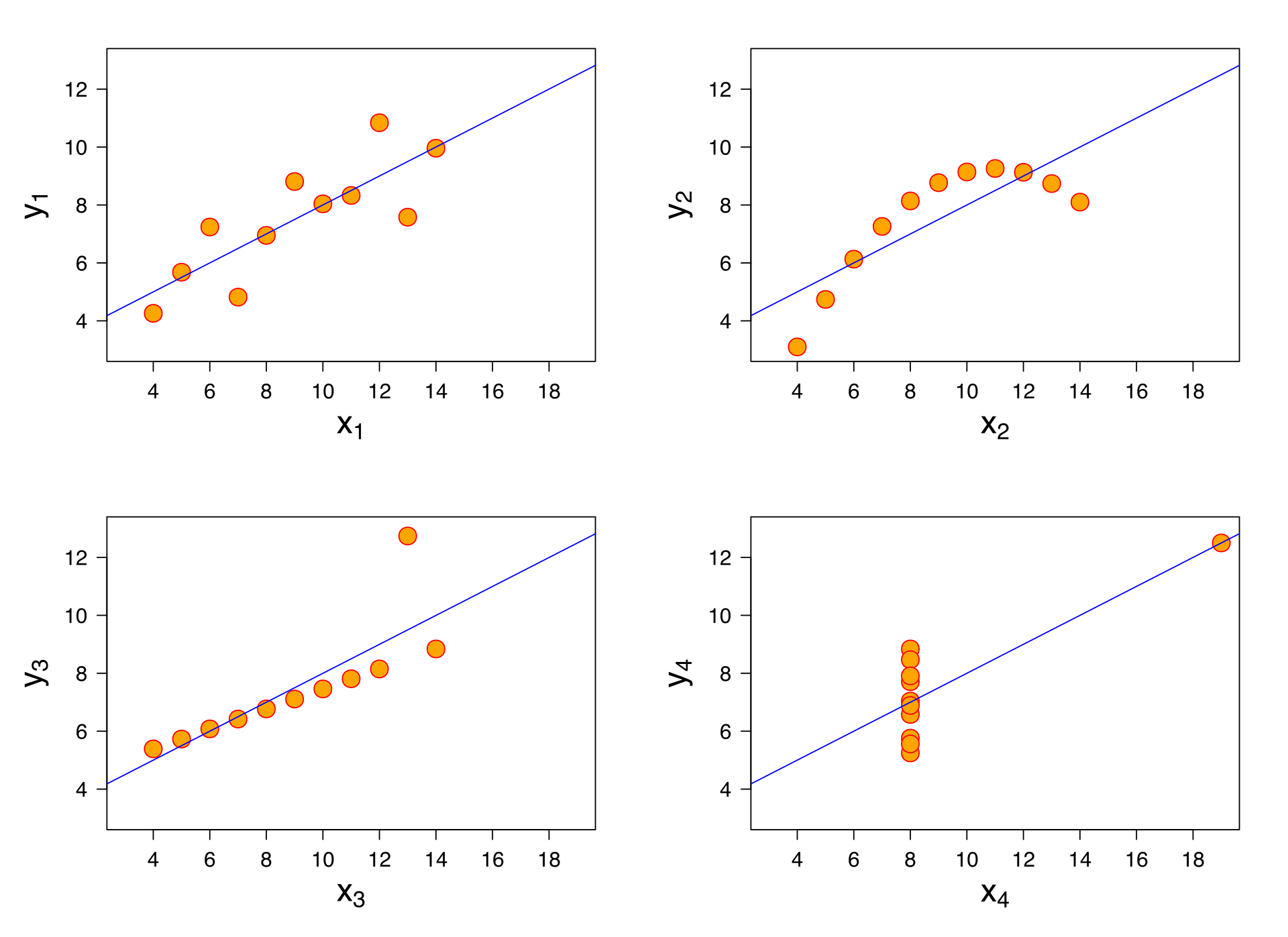
As you can see, these datasets are doing very different things, but the linear model that best describes them is the same for all four datasets. It also fits each dataset as well as the next: the \(R^2\) is \(0.67\) for all the regressions. This is a cautionary tale: sometimes a linear model is simply not the right model!
Running a linear regression on a Pandas dataframe#
Now we’re going to load another CSV; this time, it will be full of fish measurements (source) that we will attempt to correlate to the fishes’ weights.
df_fish = pd.read_csv('data/Fish.csv')
df_fish.head(5)
| Species | Weight | Length1 | Length2 | Length3 | Height | Width | |
|---|---|---|---|---|---|---|---|
| 0 | Bream | 242.0 | 23.2 | 25.4 | 30.0 | 11.5200 | 4.0200 |
| 1 | Bream | 290.0 | 24.0 | 26.3 | 31.2 | 12.4800 | 4.3056 |
| 2 | Bream | 340.0 | 23.9 | 26.5 | 31.1 | 12.3778 | 4.6961 |
| 3 | Bream | 363.0 | 26.3 | 29.0 | 33.5 | 12.7300 | 4.4555 |
| 4 | Bream | 430.0 | 26.5 | 29.0 | 34.0 | 12.4440 | 5.1340 |
First, we’ll try doing a basic regression with sklearn. We need to make two numpy arrays for the linear regression module to use. So we’re going to learn how to grab numpy arrays from a pandas dataframe. We’ll use the columns Length1, Length2, Length3, Height, and Width as our independent variables. Our dependent variable, of course, is Weight.
To get a subset of columns from a dataframe, we simply list the columns we want. then call the .numpy() function. This converts our dataframe into a numeric numpy array:
col_subset = df_fish[['Length1', 'Length2', 'Length3', 'Height', 'Width']]
x_mtx = col_subset.to_numpy()
Can you figure out how to obtain the array of fish weights?
# Your Turn!!!
Importing sklearn#
sklearn, or scikit-learn, is a Python package that has a bunch of machine learning algorithms built in. We’re going to use it to practice running linear regressions. We’re also going to import numpy, which is a great package for numerical computation and array manipulation.
from sklearn import linear_model
import numpy as np
reg = linear_model.LinearRegression()
reg.fit(x_mtx, y_mtx)
LinearRegression()
We have created a LinearRegression object, called reg. When we call the fit() method, we compute the best coefficients to multiply the values in x_mtx by to get something close to y_mtx. How good is our model? The score() method gives us \(R^2\).
reg.score(x_mtx, y_mtx)
0.8852867046546207
That’s not too bad!
Adding in Fish Species#
What if our fish are different densities depending on species? Let’s see if we can make our regression a little better. One way to do this is to introduce a categorical variable. In this case, we’ll have a column for each fish species. Its entry for each row will take the value \(1\) if the fish in that row is of that species; otherwise, it’ll be \(0\). This is really easy to do with pandas:
df_fish["fish_category"] = df_fish["Species"].astype("category")
fish_dummies = pd.get_dummies(df_fish['fish_category'], prefix='species_')
We’ve created what’s called one-hot encodings, or dummmy variables, which is great news for our fish regression! Let’s create a matrix of species dummy variables:
species_mtx = fish_dummies.to_numpy()
And now we’ll concatenate that (along the horizontal axis) to our original matrix of fish measurements:
x_new = np.hstack([species_mtx, x_mtx])
We’ll make a new regression object:
reg1 = linear_model.LinearRegression()
reg1.fit(x_new, y_mtx)
LinearRegression()
How well did we do?
reg1.score(x_new, y_mtx)
0.9360849020585846
That’s better! Adding more information doesn’t always help, but this time around it did!
Getting Fancy#
We can also use something called a kernel function to transform our linear data into higher dimensional space. Specifically, we can apply arbitrary functions to our fish data and add them to our linear regression matrices. Let’s say we have two concentric circles as a dataset:
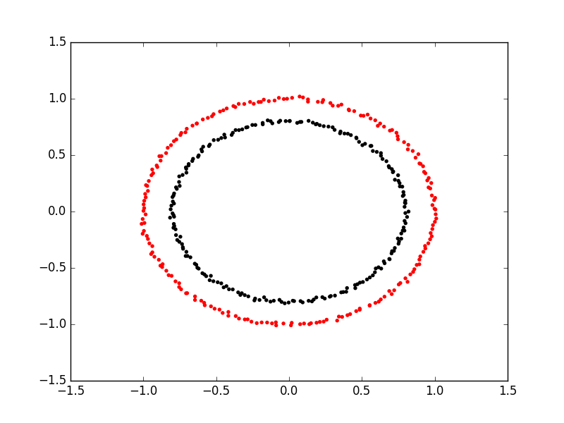 We’re going to have a hard time separating these with either of their \(x\) and \(y\) coordinates! But what if we add a new column that is \(\sqrt{x_i^2 + y_i^2}\)? We’re able to separate them easily because we’ve projected our points into a higher dimensional space. Neat!!
Let’s try applying this to the fish dataset. Can you engineer a new column for the fish dataset that improves your \(R^2\)?
# Your Turn!
Resources & Acknowledgements#
Our intro to pandas borrows heavily from 10 minutes to pandas
Our whale dataset comes from the UK Polar Data Centre
Our fish dataset is sourced from Kaggle
The kernel function image comes from the Carpentries Incubator
For more on kernel methods, check out this textbook chapter
Here’s a list of SQL commands you might want to know at some point.